Part of a series on quantitative models for cause selection.

Introduction

One major reason that effective altruists disagree about which causes to support is that they have different opinions on how strong an evidence base an intervention should have. Previously, I wrote about how we can build a formal model to calculate expected value estimates for interventions. You start with a prior belief about how effective interventions tend to be, and then adjust your naive cost-effectiveness estimates based on the strength of the evidence behind them. If an intervention has stronger evidence behind it, you can be more confident that it’s better than your prior estimate.

For a model like this to be effective, we need to choose a good prior belief. We start with a prior probability distribution P where P(x) gives the probability that a randomly chosen intervention¹ has utility x (for whatever metric of utility we’re using, e.g. lives saved). To determine the posterior expected value of an intervention, we combine this prior distribution with our evidence about how much good the distribution does.

For this to work, we need to know what the prior distribution looks like. In this essay, I attempt to determine what shape the prior distribution has and then estimate the values of its parameters.

Distribution Shape

The first question we have to ask is what probability distribution describes the space of interventions.

I see three reasonable ways to figure out the distribution:

1. Look at what properties the distribution intuitively feels like it ought to have.
2. Empirically observe interventions’ impact and fit a distribution to the data.
3. Create a theoretical model and determine its distribution.

Intuitive approach

Interventions seem to have the general property that there are a lot that have little to no effect per dollar spent, and few with large effects (as GiveWell claims here and here). In particular, the probability of finding an intervention with impact X utility diminishes as X increases.

The two most reasonable-seeming distributions with this property are the log-normal distribution and the Pareto distribution². These are by far the most common distributions that are unbounded and have long tails. If I were being more thorough I would more seriously investigate other candidate distributions, but some brief research suggests that there are no other strong contenders.

Let P(x) be a probability density function where x is a level of impact (described as a numerical utility) and P(x) gives the probability density of interventions at that level of impact. The Pareto distribution has the property that if P(x)/P(2x) = k, for some constant k, then P(ax)/P(2ax) = k for any coefficient a. This sounds like a reasonable property for the space of interventions to have.

A log-normal distribution looks similar to a Pareto distribution at some scale, but unlike a Pareto distribution, the tail diminishes increasingly quickly: for sufficiently large x, \(P_{lognorm}(x) < P_{Pareto}(x)\) no matter what parameters are used to define the two distributions.

Examples of real-world phenomena that follow a Pareto distribution include word frequency, webpage hits, city populations, earthquake magnitudes, and individual net worths³. The distribution of interventions feels qualitatively similar to these in a way that’s hard to describe. On the other hand, I don’t know of a mechanism for generating Pareto distributions that could plausibly generate a distribution of interventions (see Newman (2006)³). It seems more plausible that interventions could be modeled as a natural growth process (although I haven’t thought about this much and I’m not exactly sure how this model fits). Additionally, many data historically believed to follow a Pareto distribution were later shown to be log-normal⁴. A log-normal distribution describes such data as the lengths of internet comments, coefficients of friction for different objects, and possibly individual incomes.

Empirical approach

How can we empirically observe interventions’ impact? Can we do a good enough job to get a strong prior?

I attempted to estimate what the distribution looks like by examining the list of cost-effectiveness estimates published by the Disease Control Priorities Project. The interventions (measured in dollars/DALY) follow an exponential curve along the range [10^0, 10^4]:

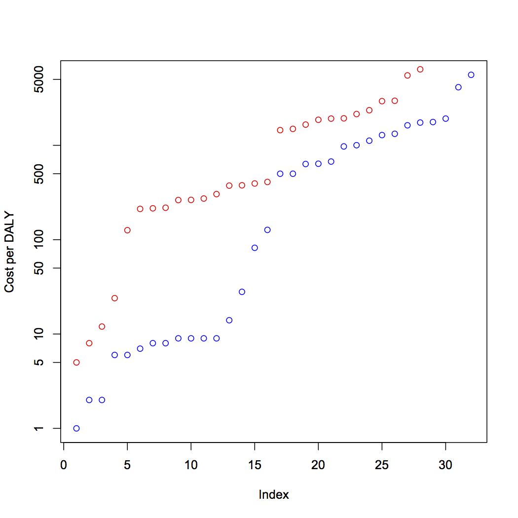
(Minimum estimates are in blue, maximum estimates are in red. Raw data available here.)

This looks sort of like what you’d get if you sampled from a log-normal distribution, but not quite. Unfortunately there are some problems with this data set:

• It’s too small to be able to make strong inferences about the shape of the distribution.
• It only includes global health interventions.
• It’s a non-random sample of interventions: it includes only those that receive sufficient attention for the Disease Control Priorities Project to evaluate.
• The included estimates might not actually be that accurate, so it might not make sense to use them to construct a prior.

What would it take to construct a true prior distribution? This would require having a large data set of random interventions where we have a fairly accurate idea of their cost effectiveness. It would probably take more work than compiling the DCP2 estimates since it would have to span a much wider scope. Perhaps a government or an organization like The Gates Foundation could construct such a data set if it put a team of researchers on the project for several years, but short of that, I don’t believe a project like this is feasible. So this approach is out. (Unless you want to do your PhD thesis on this topic, in which case I’m all for that and please send it to me once you’re done.)

Theoretical approach

Maybe we can build a theoretical model that tells us something about what we’d expect the distribution of interventions to look like.

At a naive first glance, an intervention could be anything you do that has an impact on the world. The universe is a big space and the space can be occupied by sentient beings that have positive or negative utility. So we can represent the universe as a vector where each element contains a real number representing the utility at the corresponding location in space.

The universe naturally changes over time. We can represent this change by multiplying the universe vector by a square matrix.

An intervention changes your little localized part of space and then potentially has effects that propagate throughout the universe. We can represent an intervention by adding 1 to some element of the vector.

We can find a theoretical prior distribution by looking at the distribution of utility differences when we change the elements of the universe vector. This distribution is the sum of a large number of uniform distributions, so it’s approximately normal. Does that mean we should use a normal distribution as the prior?

I don’t think so. This theoretical model is pretty coarse, and it covers the space of all possible actions rather than all reasonable interventions. There are lots and lots of things you could do to try to improve the world that you never will do because they’re so obviously pointless.

Let’s consider an alternative model where an action has some immediate impact, and then has effects that propagate outward multiplicatively. Here, if the effects propagate over sufficiently many steps, then by the Central Limit Theorem the final distribution will be log-normal. This is some evidence in favor of using a log-normal distribution as the prior.

One person I spoke to suggested that actions have some additive effects and some multiplicative effects, so the prior should look something like a combined normal/log-normal distribution. This is an intriguing idea worth further consideration, but I won’t discuss it more here.

Discussion of approaches

None of the considerations so far have been particularly strong. At this point, I weakly prefer log-normal distributions over Pareto distributions because I find it plausible that interventions follow something like a multiplicative growth process that tends to generate log-normal distributions.

Setting Parameters

We can estimate parameters by trying to figure out what’s reasonable a priori, and by picking parameters that produce reasonable results. The latter approach begs the question a bit, but I actually think it’s reasonable to use. You probably have strong intuitions about how to compare some interventions and weak intuitions about how to compare others. You can check your model against the interventions where you have good intuitions. Then you can think of the model as a formalization of your intuitions that makes it easier to extrapolate to cases where your intuitions don’t work well.

I have decent intuitions about, for example, how to trade off between GiveDirectly and the Against Malaria Foundation (AMF). GiveWell’s latest estimate (as of this writing) suggests that AMF is 11 times more cost-effective than GiveDirectly. The evidence for GiveDirectly is stronger, so I’d be indifferent between $1 to AMF and maybe $6-$8 to GiveDirectly. So I should choose parameters that get a result close to this. But I don’t have good intuitions about how good AI safety work is compared to GiveDirectly, so if I build a good model, its results will be more useful than my intuitions.

Median

Pareto and log-normal distributions both have two main parameters; we can call them the shape parameter and scale parameter (they correspond to α and x_m for Pareto, and μ and σ for log-normal). If we know the shape parameter and the median, we can deduce the scale parameter. For either distribution, it’s probably easier to guess the median a priori than to guess the scale; so let’s consider what the median should be.

The median depends a lot on what your reference class is. Are you looking at all possible actions? Almost all actions are pretty useless. Maybe instead you should look at non-obviously-useless actions. This still includes things like PlayPumps, but I don’t expect I’ll be tempted to support most of these things.

So perhaps the reference class should be the set of all interventions that I might be tempted to support (with my money or time). It seems plausible to me that GiveDirectly is about the median for this set. I wouldn’t support anything worse than GiveDirectly on purpose, but a lot of things that I think might be effective probably aren’t that effective. Unfortunately, this decision is pretty arbitrary and I see no obvious way to make it more well-informed. Fortunately, the choice of the median doesn’t have as big an effect as the choice of the shape parameter.

Reverse-Engineering Parameters

Let’s look at three example interventions. Say we have GiveDirectly with an estimated utility of 1, Against Malaria Foundation with an estimated utility of 11, an animal advocacy intervention with estimated utility 2x10⁴, and an x-risk intervention with estimated utility 10⁴⁰ (these estimates come from my previous essay). Let’s look at how the posterior expected value changes as we vary the s parameter for the estimate and the parameters for the prior distribution. I chose values (0.1, 0.3, 0.8, 2.0) because I believe these are approximately the order-of-magnitude standard deviations on the estimates for GiveDirectly, AMF, animal advocacy (in particular corporate campaigns), and x-risk (in particular AI safety) respectively⁵.

The results for a Pareto prior scale x_m such that the prior distribution has a median of 1.

The results for a log-normal prior use median 1 and vary the σ parameter. (σ in the prior represents the same thing as s in the estimate.)

Pareto prior

α = 1.1:

s	GiveDirectly	AMF	animals	x-risk
0.10	1.03	10.77	1.94e+04	9.69e+39
0.30	1.22	9.36	1.50e+04	7.51e+39
0.80	2.09	6.67	2667.24	1.31e+39
2.00	4.32	6.60	45.21	2.98e+34

α = 1.5:

s	GiveDirectly	AMF	animals	x-risk
0.10	1.03	10.63	1.90e+04	9.48e+39
0.30	1.23	8.51	1.24e+04	6.21e+39
0.80	1.92	4.99	743.02	3.36e+38
2.00	2.83	3.69	10.10	6.16e+30

α = 2.0:

s	GiveDirectly	AMF	animals	x-risk
0.10	1.03	10.47	1.85e+04	9.24e+39
0.30	1.24	7.74	9780.87	4.89e+39
0.80	1.80	4.02	185.91	6.16e+37
2.00	2.25	2.74	5.23	1.53e+26

s	GiveDirectly	AMF	animals	x-risk
0.10	1.03	10.21	1.75e+04	8.76e+39
0.30	1.25	6.78	6076.03	3.03e+39
0.80	1.68	3.24	33.64	2.07e+36
2.00	1.88	2.19	3.42	9.42e+16

Log-normal prior

σ = 0.5:

s	GiveDirectly	AMF	animals	x-risk
0.10	1.00	10.03	1.37e+04	2.89e+38
0.30	1.00	5.83	1453.86	2.58e+29
0.80	1.00	1.96	16.15	1.72e+11
2.00	1.00	1.15	1.79	225.39

σ = 1.0:

s	GiveDirectly	AMF	animals	x-risk
0.10	1.00	10.74	1.81e+04	4.02e+39
0.30	1.00	9.02	8828.75	4.98e+36
0.80	1.00	4.32	419.35	2.46e+24
2.00	1.00	1.62	7.25	1.00e+08

σ = 1.5:

s	GiveDirectly	AMF	animals	x-risk
0.10	1.00	10.88	1.91e+04	6.65e+39
0.30	1.00	10.03	1.37e+04	2.89e+38
0.80	1.00	6.47	2231.27	1.39e+31
2.00	1.00	2.37	35.35	2.51e+14

Observations

• Based on the results for AMF and animals, α = 3.0 and σ = 0.5 look the most reasonable. For a Pareto prior we might even want to go higher than α = 3.0.
• Under a Pareto distribution, as s increases, posterior EV drops very suddenly on a log scale (e.g. 10³⁹, then 10³⁹, then 10³⁷, then 10²⁶). Under a log-normal distribution, as s increases, posterior EV drops fairly smoothly. I have a sense that the log-normal behavior is better here but I don’t really know.
• Basically, for short-term interventions, parameter choice matters more than distribution shape. The distribution shape only has a really big effect when you look at x-risk, which is orders of magnitude larger and have much higher variance.

Setting Different Priors for Different Interventions

This all assumes that we’re using a single prior for all interventions. But perhaps global poverty and x-risk are sufficiently different that we should use different prior distributions for them.

Now, I’m somewhat wary of using different priors for different interventions because it makes it easier to tweak the model to get the results you want, but I believe we can avoid this if we’re careful. Instead of changing priors based on whatever seems reasonable, which leaves lots of room for biases to creep in, we can change priors in a systematic way.

I believe the following system is defensible:

1. Changing σ across priors is too subjective and has a lot of room for bias, so let’s keep it fixed.
2. It’s possible to have a larger effect when helping a group that people with power care less about.

To expand on point 2: most people with power⁶ care about other people in the developed world more than people in the developing world, because people in the developed world tend to have more power and they care more about themselves and people around them. Even within the developed world, rich people are harder to help than poor people because rich people already have a lot of resources.

People care even less about non-human animals, beings in the far future, and sentient computer simulations. So we should expect on priors that these groups are easier to help.

Even without knowing anything about particular animal advocacy interventions, I would expect that the best ones are better than the best global poverty interventions, because I believe most people with power irrationally discount non-human animals in the same way they irrationally discount humans in the developing world.

GiveWell’s estimates suggest that it’s more than an order of magnitude more expensive to help humans in America than humans in the developing world.It’s probably reasonable to assume that it’s 10 times easier to help non-human animals than humans, since philanthropists care much less about non-human animals than about humans and animal advocacy receives far less funding than global poverty. We could use something like the following medians for prior distributions in different categories:

Category	Median
developed-world poor	0.1
global poor	1
factory-farmed animals	10
far future humans	10
wild animals (now and far future)	100
sentient computer programs	100

People will inevitably disagree on these priors. I’m sympathetic to the case for making all the priors the same, but I’m also sympathetic to the case for making the differences in priors a lot wider.

Conclusions

I have an intuition that the probability of observing an intervention with expected value 2X is a constant fraction of the probability of observing an intervention with expected value X, no matter the value of X. The only distribution with this property is a Pareto distribution. When I first wrote this post I felt that a Pareto distribution described the prior well, but after looking at the data more, I believe a log-normal distribution works better. I don’t find it plausible that I should be indifferent between $1 to AI safety and $94,200,000,000,000,000 to GiveDirectly⁷, as a Pareto prior suggests. And because of the shape of a Pareto distribution, you can’t fix this by reducing the variance of the prior unless you reduce it to an absurdly small number. On the other hand, this isn’t great reasoning and I have a lot of uncertainty here.

For a log-normal prior, choosing parameter σ = 0.5 and putting GiveDirectly at the median produces more reasonable results than other obvious parameter values. I will use σ = 0.5 in future essays that require using a prior distribution. Once it’s more polished, I will provide the spreadsheet I used to do these calculations; if you believe σ = 0.5 produces results that penalize high-variance interventions too much or too little, you can increase or decrease σ accordingly.

I believe the most difficult and important choice here is what distribution shape to use for the prior, and I do not believe any of the evidence I presented here is particularly strong. I’m interested in hearing any arguments for why we should use Pareto, log-normal, or something else.

Thanks to Gabe Bankman-Fried and Claire Zabel for providing feedback on this essay.

Notes