Confidence: Likely.

If you take caffeine every day, does it stop working? If it keeps working, how much of its effect does it retain?

There are many studies on this question, but most of them have severe methodological limitations. I read all the good studies (on humans) I could find. Here’s my interpretation of the literature:

• Caffeine almost certainly loses some but not all of its effect when you take it every day.
• In expectation, caffeine retains 1/2 of its benefit, but this figure has a wide credence interval.
• The studies on cognitive benefits all have some methodological issues so they might not generalize.
• There are two studies on exercise benefits with strong methodology, but they have small sample sizes.

Clarifying terminology

The scientific literature talks about the “caffeine withdrawal hypothesis.” People use this term to describe two very different hypotheses:

1. Caffeine has no benefits for anyone. It reverses withdrawal symptoms for habituated users, but it doesn’t do anything for non-users. (Call this the “caffeine-is-useless hypothesis.”)
2. Caffeine initially has benefits for non-users, but if you use caffeine habitually, your body adjusts to the point where you need caffeine just to get back up to baseline. (Call this the “caffeine habituation hypothesis.”)

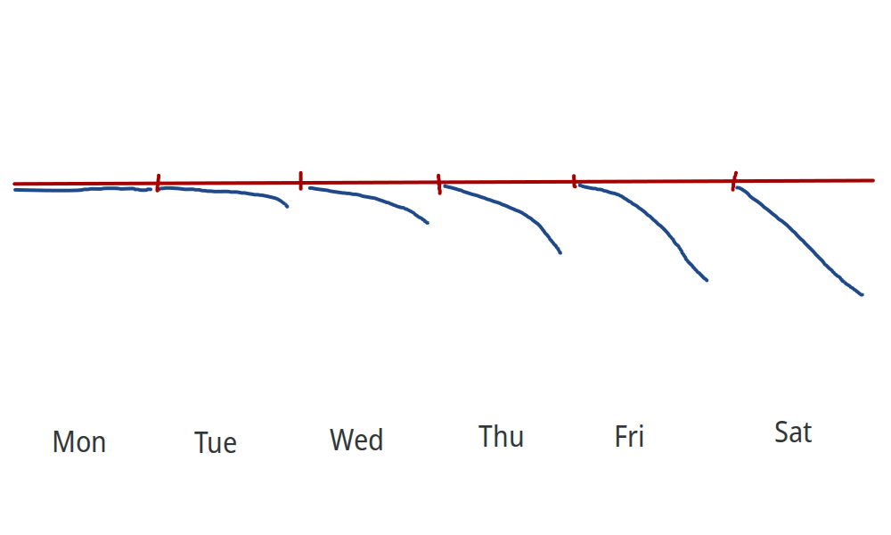
According to the caffeine-is-useless hypothesis, on the first day you take caffeine, you experience no benefits, and then you start feeling withdrawal symptoms after you’ve been taking caffeine for a few days:

According to the caffeine habituation hypothesis, caffeine has initial benefits, but you start developing a tolerance:

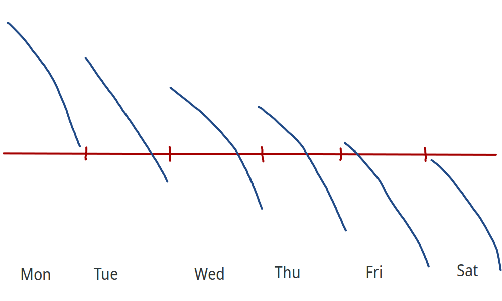
(Graphs inspired by Gavin Leech’s article on caffeine, except I put way less effort into mine.)

Most studies on caffeine withdrawal only look at the caffeine-is-useless hypothesis. The study results pretty much universally reject this hypothesis so I consider it roundly falsified¹. I’m much more interested in the caffeine habituation hypothesis, so that’s the one I will be discussing.

Research papers almost never explicitly discuss the caffeine habituation hypothesis, but some of them provide enough data to test it. In the next two sections, I will review some studies and figure out what their data tell us about the caffeine habituation hypothesis.

Cognition studies

I found two good studies on the exercise benefits of caffeine, and four good(ish) studies on the cognitive benefits. Let’s start with the cognition studies: Rogers et al. (2013)², Hewlett & Smith (2007)³, Haskell et al. (2005)⁴, and Smith et al. (2006)⁵.

These studies all used similar methodology: they divided participants into high caffeine users vs. low/non-users. Then they randomly administered either caffeine or placebo and tested participants’ performance on various cognitive tests.

The studies each have four groups of participants:

1. LoCaf: low- or non-caffeine users assigned to take caffeine
2. LoPla: low- or non-caffeine users assigned to take placebo
3. HiCaf: high-caffeine users assigned to take caffeine
4. HiPla: high-caffeine users assigned to take placebo

To test the caffeine habituation hypothesis, compare the performance of high-caffeine users after taking caffeine (HiCaf) versus low-caffeine users after taking placebo (LoPla). If high users develop complete tolerance then these two groups should perform the same: when a habitual user takes caffeine, it brings their performance back up to baseline, but has no benefits beyond that.

(This methodology isn’t perfect because low and high caffeine users might differ in ways that could bias the results.⁶ (For more discussion of this possibility, see Rogers et al. (2013)².) It would be better to randomize participants to take either caffeine or placebo for several weeks.)

Then calculate:

• baseline benefit = LoCaf – LoPla = benefit to a naive user
• habituated benefit = HiCaf – LoPla = benefit to a habituated user
• retention = habituated benefit / baseline benefit = (HiCaf – LoPla) / (LoCaf – LoPla) = what proportion of caffeine’s benefits are retained by a habituated user

Retention ranges from 0 (caffeine loses all its effect) to 1 (caffeine retains all its effect).

I evaluated the effectiveness of caffeine by computing approximate likelihood functions of retention from each study’s measurements.

(Disclaimer: I only just now learned how likelihood functions worked so I could write this article. Be wary of mistakes.)

The likelihood function L(X) answers the question, “If caffeine’s true retention is X, what is the probability that we would measure the retention that we did in fact measure?” If a particular retention has a high likelihood of generating the results we got, that makes it more likely that that’s the true retention.

(For a longer explanation of likelihood functions, see Report Likelihoods, Not P-Values.)

Plotting likelihood functions of the four main metrics⁷ from Rogers et al. (2013) (which had a larger sample size than the other three studies combined) along with the average likelihood⁸ of those metrics:

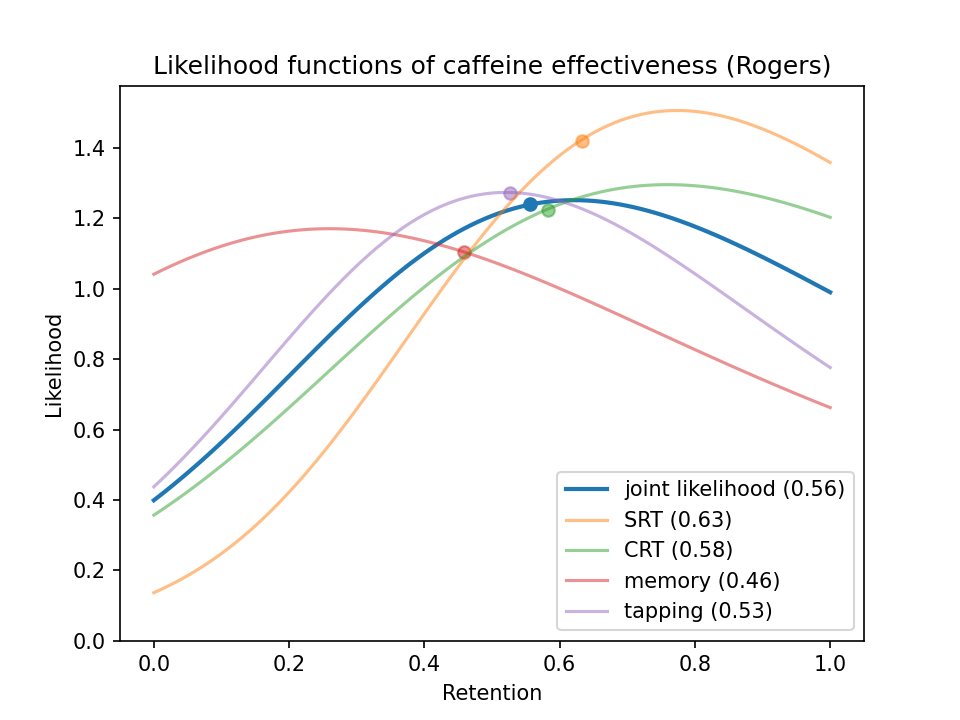
(The dots on each curve show the mean likelihoods. You can interpret the mean as the value the evidence tends to point toward.⁹)

This graph says the experiment points toward caffeine retaining around half its effect (0.56 to be precise). And it says we’d be somewhat unlikely to see these experimental results if retention = 0, but not unlikely to see them if retention = 1.

Here’s how I computed these approximate likelihood functions:

Model the baseline benefit (LoCaf - LoPla) and habituated benefit (HiCaf - LoPla) as t-distributions.¹⁰ To compute the likelihood function for retention (habituated benefit / baseline benefit), we need to know the shape of a ratio of t-distributions.

A ratio of t-distributions does not have a closed form solution. So I approximated the solution using a formula I pulled off Wikipedia for the ratio of two independent normal distributions (astute readers will notice that the distributions in question are neither independent nor normal). I guess you could call this the Simon-Ftorek approximation because Wikipedia cites Simon and Ftorek (2022)¹¹. For more on whether this approximation is any good, see Appendix A.

I used the Simon-Ftorek approximation to compute the likelihood functions for the most important metrics in each study (see Appendix B for a list of all the metrics I used). Then I computed a likelihood function for each study as the (geometric) average of all the likelihood functions for individual metrics in that study. Normally, you’re supposed to compute a joint likelihood as the product of your likelihood functions. But that assumes each function provides independent evidence, and I figured if you have the same study with the same participants, the different metrics all basically represent the same evidence. So I averaged them instead of multiplying them.

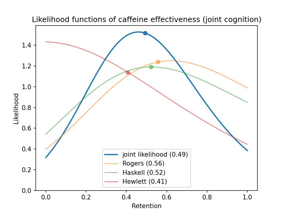
If we take the joint likelihoods from the four cognition studies and combine them into one big joint likelihood, we get this:

Exercise studies

I found two good studies on how habitual caffeine affects exercise: Beaumont et al. (2017)¹² and Lara et al. (2019)¹³. These two studies had participants abstain from caffeine for a month. Then they gave participants either caffeine or placebo for several weeks, testing their exercise performance at the beginning and end of the study.

The methodologies different somewhat, and I calculated retention accordingly.

In Beaumont et al. (2017)¹², the participants took two pre-tests, one with caffeine and one with placebo. Then after taking caffeine every day for 28 days, they took a dose of caffeine and a final performance test. I calculated

• baseline benefit = caffeine pre-test – placebo pre-test
• habituated benefit = caffeine post-test – placebo pre-test
• retention = habituated benefit / baseline benefit

Lara et al. (2019)¹³ tested participants 3 times a week for 20 days. To take advantage of all the extra data points, I plotted a linear regression over the performance for the caffeine group minus the placebo group¹⁴. Then I calculated

• baseline benefit = projected effect size on day 0 (= intercept of the regression)
• habituated benefit = projected effect size on day 20
• retention = habituated benefit / baseline benefit

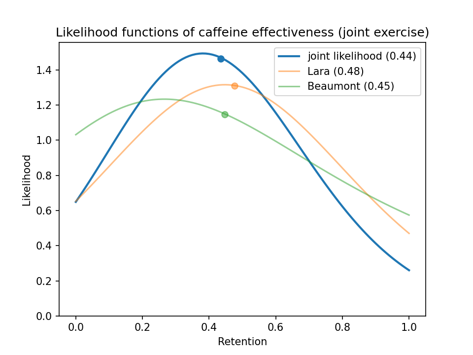
It looks like caffeine doesn’t fare as well for exercise as for cognition—it only retains about 1/3 of its effect. (But both exercise studies were underpowered so we can’t say that with much confidence.)

Some problems with my approach

• As I mentioned before, I couldn’t calculate exact likelihood functions, I could only approximate them.
• I assumed caffeine has the same effect on all cognitive tests and on all exercise tests. But caffeine probably helps more with some tasks than others. It probably improves reaction time more than memory; it probably helps more with sustained moderate exercise (e.g., a VO2 max test than with short intense efforts (e.g., a Wingate test).
• Limiting the domain to [0, 1] makes the likelihood means tend toward 0.5 because it chops off the (often large) parts of the distribution below 0 and above 1. If you think retention can go above 1 but not below 0, you’ll get a higher mean. Conversely, if you think it can go below 0 but not above 1, you’ll get a lower mean. (Symmetrically expanding the domain to [-1, 2] doesn’t change the answers much.)

Conclusion

I plotted likelihood functions for every I study I reviewed and combined them into one big joint likelihood:

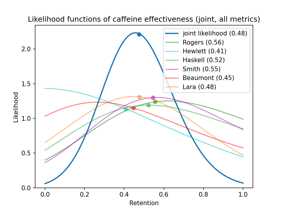
What about a posterior probability?

If you use a uniform prior for caffeine retention, the posterior probability distribution simply equals the likelihood function. According to the studies I looked at, a habituated caffeine user retains an expected 49% of the cognitive benefit and 44% of the exercise benefit, or 48% if we combine the cognition and exercise studies.

My prior has more probability mass near 0 than 1. Human bodies want to maintain homeostasis, so there’s some theoretical reason to expect your body to adjust until caffeine stops working entirely. (And, empirically, taking caffeine does cause your brain to grow more neurotransmitter receptors,¹⁵ although it’s not clear how this corresponds to cognitive function.) Changing the prior moves my posterior expected retention from 48% to 43% or so.¹⁶

As shown in Appendix A, my approximation for the likelihood function understates the mean. Plus my review excluded any metrics where caffeine had too small a baseline benefit, which biases the retention to look smaller. Due to these factors, the true implied retention is higher than 43%. Let’s call it 50% to make it a nice round number.

So we can reasonably say, albeit with a high degree of uncertainty, that caffeine retains something like half its benefit for a habitual user.

Source code for my calculations can be found on GitHub.

Appendix A: Approximating the retention ratio

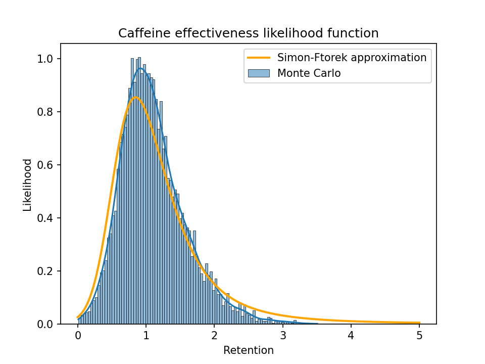
As a sanity check, I generated 10,000 random samples following the same distribution as the groups in one of the caffeine studies (Rogers et al. (2013)²), where each sample represents a set of true parameter values that could correspond to the observed values for the four groups (LoCaf, LoPla, HiCaf, HiPla). Then I calculated the distribution of true retention and the Simon-Ftorek approximation of the likelihood function (normalized to integrate to 1) and plotted them together:

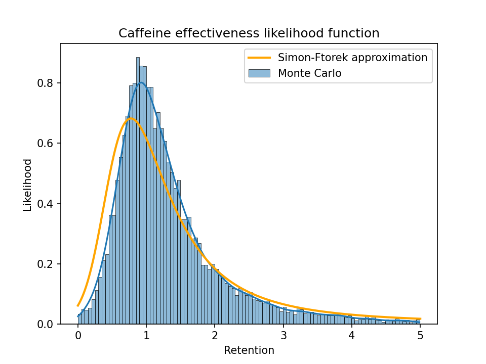
A zoomed-in plot showing just the values from 0 to 1:

(The upper plot already chops off a big tail. The largest retention value in the sample was over 500, i.e., a long-term caffeine user appears to get a 500x larger benefit per dose than a naive user. That can happen with a ratio of random variables when the denominator ends up close to 0.)

From these plots we can see that a Simon-Ftorek approximation slightly overstates the width of the distribution.

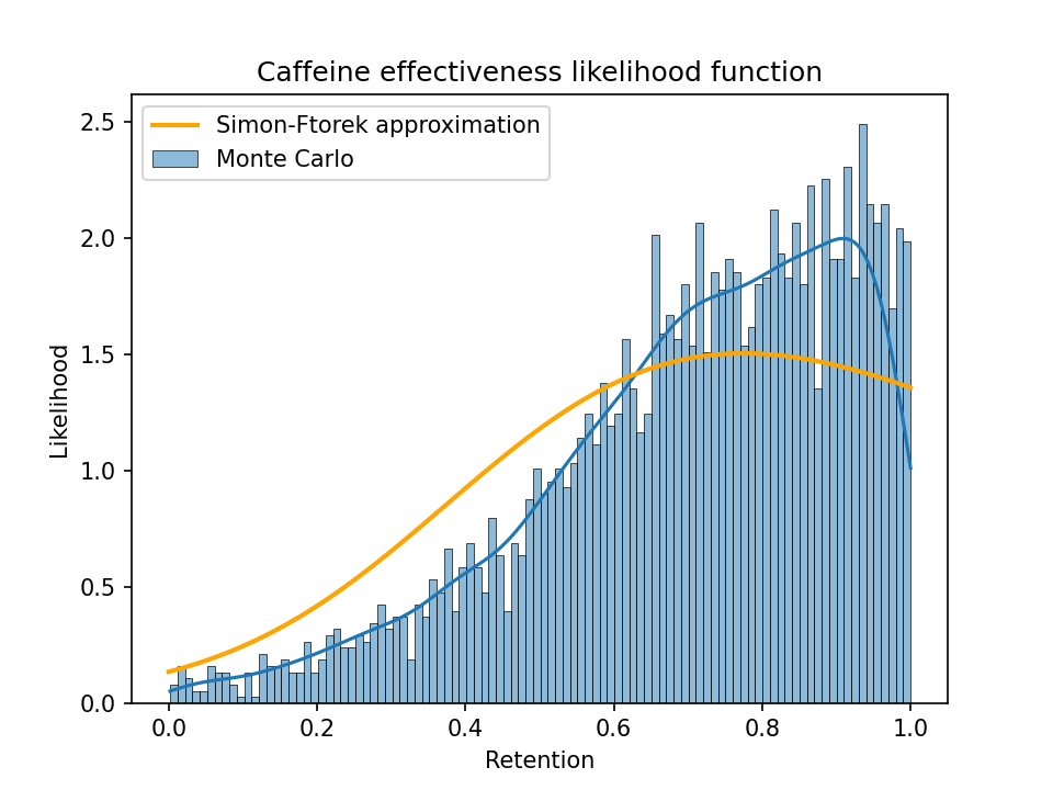
If we restrict the Monte Carlo sample to just the results with a baseline benefit of least one standard error (as I did when selecting metrics to look at), we get this:

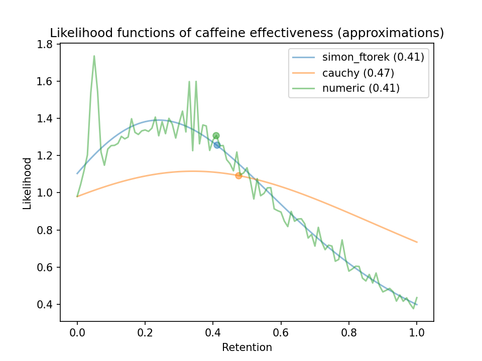
I also tried two other approximations, but Simon-Ftorek seemed best. The other approximations I tried:

• Approximate using a Cauchy distribution. A Cauchy distribution perfectly represents the ratio of two central normal distributions, so I figured it might be an okay approximation for the ratio of non-central normal distributions.
• Numerically compute the ratio of two distributions represented as histograms. This still requires assuming the distributions are independent.

This plot shows the three different approximations over a single metric from Beaumont et al. (2017)¹²:

Appendix B: List of all metrics used

I did not use metrics from every study. I used the following criteria to select metrics:

• Only use performance metrics, not subjective ratings or physiological measurements. (That means no sleepiness, no heart rate, etc.).
• Prefer metrics that the study authors emphasized.
• Don’t use any metrics where the baseline benefit was small (<1 standard error) or negative.

I used the following metrics from each study:

• Rogers et al. (2013)²: simple reaction time, choice reaction time, recognition memory, tapping speed
• Hewlett & Smith (2007)³: focused attention speed, simple reaction time, verbal reasoning % correct
• Haskell et al. (2005)⁴: simple reaction time, digit vigilance reaction time, Rapid Visual Information Processing false alarms, spatial memory (sensitivity index), numeric memory reaction time
• Smith et al. (2006)⁵: focused attention speed, categoric search reaction time, simple reaction time, vigilance hits
• Beaumont et al. (2017)¹²: total energy output (kJ), substrate oxidation
• Lara et al. (2019)¹³: peak power, VO2 max, Wingate test peak power, Wingate test mean power

Smith et al. and Lara et al. did not provide numeric standard errors (and Lara et al. did not provide means) but did provide plots, so I estimated the numeric values by counting the number of pixels using Gimp.

Note: Ignoring metrics with a small or negative baseline benefit could bias the results toward making caffeine habituation look worse. This process selects for observations where the baseline benefit was large by chance, making the habituation benefit look smaller by comparison.

Notes