Should Global Poverty Donors Give Now or Later?
Update 2020-01-04: This essay contains a number of important mistakes. See Correction on Giving Now vs. Later.
Disclaimer: I am not an investment advisor and nothing in this essay serves as investment advice.
Introduction
Robin Hanson: If More Now, Less Later
The rate of return on investment historically has been higher than the growth rate–or, as they say, r > g. If you save your money to donate later, you can earn enough interest on it that you eventually have the funds to donate a greater amount. Because r > g, you should invest your money for as long as you can before donating1–or so the argument goes.
Traditionally, we’d apply a discount rate of g to future donations, because that’s the rate at which people get richer and therefore the rate at which money becomes less valuable for them. But this ignores some important factors that affect how much we should discount future donations, and we can create a much more detailed estimate. This essay will explore that in detail. Exactly what factors determine the investment rate of return and the discount rate on poverty alleviation? Can we gain any information about which is likely greater?
- Introduction
- Basic formulas for the investment rate of return and the discount rate on poverty alleviation
- Input variables, and what values they might take on
- Tentative Results
- Extra Details
- Qualitative factors may tilt the scales toward giving now
- There are three main ways of giving later, all of which have problems
- Investing looks particularly bad right now, but only under certain assumptions
- Should you give later if you expect investment returns to improve?
- What if donations produce compounding returns?
- Existential risk makes giving later look worse
- If the best global health interventions are getting used up (a.k.a.
d > 0), why hasn’t the bottom decile experienced greater income growth?
- Concluding Remarks
- Notes
What this essay is not:
- A look at giving now vs. later for any cause area other than global poverty. other cause areas have different considerations, and including them would make this essay too long. I plan to write a future essay on giving now vs. later for existential risk.
- A consideration of personal or social factors on giving now vs. later. This essay only examines the investment rate of return versus the discount rate on global poverty donations. (I would have used that last sentence as the title, but it’s too long.) For some broader considerations on giving now vs. later, see Julia Wise’s Giving Now vs. Later: A Summary.
The problem under discussion–comparing the investment rate of return and the discount rate on poverty alleviation–raises a great many questions, and these questions raise their own questions, branching out into an ever-growing tree. I do not claim to address every relevant consideration; I merely consider this essay one possible take on the problem. I have considered many counterarguments to various claims this essay makes, but left out many of them for the sake of (relative) brevity.
Basic formulas for the investment rate of return and the discount rate on poverty alleviation
This section provides formulas for the investment rate of return and the discount rate on poverty alleviation, along with the reasoning for selecting those particular formulas.
We can write the investment rate of return as:
Where:
g= GDP growthi= investment income (dividends, rents, etc.)v= valuation-
`α` (alpha) = extra return on top of the market rate
A formula for the discount rate on poverty alleviation:
Where:
g= GDP growthq= income inequality reduction rate, a.k.a. the growth rate of the global poor relative to world GDP growth (note that this could be negative)d= rate at which the best giving opportunities dry up over time, on top ofq
In plain English, g + q represents the income growth rate of the poorest people in the world. We can break this down into world GDP growth plus the additional growth (or contraction) that the global poor experience. The discount rate on unconditional cash transfers is given by g + q, for reasons discussed below. If we can find more cost-effective giving opportunities than cash transfers, we should discount them at rate p = g + q + d.
Why this formula for r?
The simple version of the formula for return on capital is r = g + i. In the long run, asset prices increase at the same rate as GDP (g), and the assets pay out income (i), so the total return is asset price growth (=GDP growth) plus income.
This must hold in the long run (as explained below), but in the short run, the market can drift above or below its intrinsic valuation. The v term accounts for these fluctuations: if the market currently trades below intrinsic value then v will be positive, and vice versa.
Do asset prices really grow with GDP?
The current price of a capital-generating asset (such as a stock) represents the market’s prediction of the discounted present value of all future income for that asset. The investment income i grows approximately with GDP2, so the discounted value of all future income payments must grow at the same pace.
Consider what would happen otherwise, if a stock’s dividend yield permanently increased faster than its stock price. Eventually the stock would pay out some absurdly high dividend like 100% (i.e., you can double your money in a year by buying the stock). If a stock’s dividend yield gets too high, investors will rush in to buy it, thus driving up the price.
But that’s just an argument, and you can prove anything with arguments. So let’s use an appeal to authority instead. Warren Buffett said that the ratio of market capitalization to GDP “is probably the best single measure of where valuations stand at any given moment.” In other words, he believes that the market’s intrinsic valuation is tied to GDP. If it goes much higher or lower then it’s probably over- or under-valued.
Note that over short time periods, asset prices need not grow with GDP. They may become detached from their intrinsic value, but they will eventually mean revert. The v term in the return-on-investment formula accounts for this. For example, the United States greatly deviated from intrinsic value in the 2000 dot-com bubble, so the rate of return in 2000 would have included a large negative value for v (when valuations are high, future return expectations are correspondingly low).
Why apply an exponential discount rate to global poverty alleviation?
An exponential discount rate p relies on the core assumption that increasing someone’s income by a certain percentage does the same amount of good no matter their absolute income level–if someone’s twice as rich, you need to give them twice as much money to produce the same increase in welfare. In other words, utility is logarithmic with income. This assumption probably isn’t strictly true, but it’s pretty close. It fits the (admittedly limited) empirical data3, and it’s built in to a lot of common assumptions we make.
Consider what the world would be like if utility were not logarithmic with income.
- Suppose utility is linear with income. That means there’s no reason to donate to charity because rich people get just as much value out of each extra dollar as poor people do. In fact you should really donate your money to hedge fund managers because they can use your money to make even more money for themselves.
- Or maybe, as they say, “Money cannot buy happiness.” In that case you might as well burn all your money because it won’t make you or anyone else happy.
Clearly our reality looks nothing like the linear-utility or the zero-utility world. On the other hand, people’s behavior generally makes sense if money provides logarithmic utility.
If we want to get a little more into the weeds, we could argue about whether we should care about log wealth instead of log income. That’s a big question, and it probably doesn’t have much bearing on our ultimate decisions so I’m not going to get into it. For our purposes, we can consider income and wealth roughly equivalent. Similarly, I conflate income and consumption; these are sufficiently similar that conflating them is a broadly accepted practice.
Why is the discount rate on cash transfers given by g + q?
To start, let’s use GiveDirectly as our model charity. It gives cash directly to the global poor. Some charities may do more good per dollar than GiveDirectly, and we will discuss that possibility; but probably no global poverty charity does much better, so GiveDirectly serves as a reasonable baseline.
For GiveDirectly, d = 0 in our formula p = g + q + d, so for now we can simplify it to p = g + q: we discount future donations to GiveDirectly according to the income growth rate of the poorest people in the world.
If we assume that utility scale logarithmically with income, the good we can do with a cash transfer depends on the ratio of the size of the donation to the income of the recipient. The return on investment r determines how much more you can donate in the future if you invest your money. While you’re holding your investments, the world’s poorest people get richer at rate g + q: the global GDP growth plus the rate of inequality reduction (or inequality increase, if q is negative). If the global poor are gaining wealth more quickly, that means your future donations won’t matter as much to them; and vice versa.
g + q is what’s called the “anonymous” income growth rate. It doesn’t tell us the rate of income growth for a particular poor person; instead, it tells us the rate at which the poorest (say) 10% of people get richer, even if the poorest 10% at one time are different people from the poorest 10% at another time. For example, in the 80’s and 90’s, most of the people in the bottom decile of income lived in India and China; but today they’re mainly in sub-Saharan Africa4. That means the poorest Chinese experienced income growth greater than g + q, while the poorest Africans did relatively worse.
We care specifically about anonymous income growth (g + q) rather than non-anonymous growth (e.g., the growth rate of the poorest people in China in particular) because giving opportunities scale with g + q. Currently, GiveDirectly primarily serves people in Kenya; but if poor Kenyans move up on the income scale and thus cash transfers become less effective for them, GiveDirectly can go find the new poorest people and give cash transfers to them instead.
Should we consider the relative income growth of the top 1%?
Given that most of my readers are in the global top 1%, and many are in the top 0.1%, we might think it pertinent to consider the rate of income growth among the richest people in the world–higher relative growth means we can expect the size of our donations to grow more quickly than world GDP and thus do more good in the future. But this isn’t particularly relevant. If you save money to donate later, you cannot invest that cash directly into your own income; you can only invest it in, well, investments.
That said, you may at some point in your life have a choice between donating money now or spending money to benefit your career growth, in which case you do care about how quickly you expect your salary to increase. You can probably get much better information about projected salary growth by looking at statistics for your field and examining your particular situation than you can by looking at global income growth statistics. I won’t consider this in detail, but if you want, you can consider investing in personal development as a form of investment and re-calculate r based on this.
Giving opportunities may disappear faster than g + q
To quote Scott Alexander, paraphrasing Elie Hassenfeld: “in the 1960s, the most cost-effective charity was childhood vaccinations, but now so many people have donated to this cause that 80% of children are vaccinated… In the 1960s, iodizing salt might have been the highest-utility intervention, but now most of the low-iodine areas have been identified and corrected. While there is still much to be done, we have run out of interventions quite as easy and cost-effective as those. And one day, God willing, we will end malaria and maybe we will never see a charity as effective as the Against Malaria [Foundation] again.”
The world’s poorest people may experience improvements to their lives more quickly than their income grows. Or it may become more difficult to find people who we can easily help. For whatever reason, cost-effective giving opportunities may disappear faster than g + q, so we should apply an extra discount rate d.
Input variables, and what values they might take on
Recall our two formulas:
Let’s consider each term in these formulas and discuss what values it might reasonably take on.
Investment rate of return, excluding α
The global stock market has experienced a long-run real return of about 5%5. A lot of people quote 7% as the long-run return, and it’s true that the US stock market has returned 7% over the past 100 years or so. But the United States experienced stronger growth than any other country in the past century and we should not necessarily expect that trend to continue. So I will use the global 5% figure. This 5% can be broken down into approximately 2% GDP growth (see World Bank data) and 3% investment income.
Over time periods of about a decade, the market predictably deviates from the long-run return. The dividend discount model can be used to predict future market returns. Although the market fluctuates a lot from year to year for various reasons, the dividend discount model has reasonably strong predictive power over a 10-year timespan. Valuation metrics such as the 10-year CAPE ratio have predictive power as well. We can use these 10-year projections to decide whether to give now or later and then re-assess the projections every few years and change our policy accordingly.
The financial firm Research Affiliates produces expected 10-year returns for a variety of asset classes using similar methodology to what I described. They predict future stock returns as a combination of capital growth (same as my g), average net yield (i), and valuation change (v). As of when I’m writing this, Research Affiliates predicts g = 1.3%, i = 2.4%, and v = -1.2% for an aggregate real return of r = 2.6%.
Research Affiliates gives some assets a better 10-year expected return than stocks. EAFE (that is, the developed-country markets in Europe, Australia, and the Far East) has a projected 10-year average real return of 4.7%, and the firm predicts emerging markets to return 6.8%. You could certainly argue that potential donors ought to invest their funds in emerging markets to get higher returns (I personally put a sizable portion of my investments into emerging markets). But we can take the world stock market as the default investment.
How big is α?
`α` tells us the margin by which we can expect to outperform the market. Conservatively, we can assume that `α = 0`, but it might plausibly be greater than 0. How much greater?
Thomas Piketty claims6 that the richest 0.1% or so can earn 2-3 percentage points better returns than the market, primarily because they have access to more investment opportunities and they can hire the best money managers. As a baseline, wealthy, sophisticated investors can perhaps expect to earn an extra 2-3% return.
Financial research from Meb Faber5 as well as from Gray, Vogel, & Foulke7 show that historically, investors could have returned 4-6% alpha on top of the market return (after expenses). Market-beating strategies tend to disappear as they are discovered, but Gray et al. present reasons why they expect this not to happen (see also this talk by Wesley Gray (the relevant portion starts at 21:18)).
My own independent backtests (unpublished, based on CRSP/Compustat price and fundamentals data) suggest that small investors, by following strategies outlined by Gray et al. but buying smaller stocks, historically could have increased their alpha to about 8-10% after expenses. (Large investors cannot take advantage of this because they can’t put too much money into small stocks without moving the market.) Going forward, I expect these strategies to work less well, although probably still better than the broad market, for reasons discussed by Gray.
If you can identify the smartest people in the room (such as Warren Buffett in the 50’s, or James Simons or Joel Greenblatt in the 90’s) and get them to invest your money, you may be able to achieve even better returns. The tricky part is identifying those people in advance and being in a position where they are willing to take your money. It’s probably safe to assume that you can’t do that, but if you can, then that’s a strong consideration in favor of saving your money to donate later. Warren Buffett is almost certainly doing more good by donating $80 billion today than if he had donated a few million dollars in the 60’s.
Is the inequality reduction rate positive or negative?
In our formula for global poverty alleviation, p = g + q, the q represents the inequality reduction rate: the rate at which the poorest people’s income grows faster than world GDP (g)8. (Note that q could be negative, i.e., global income inequality could be rising.) What is the value of q?
According to GiveWell, GiveDirectly recipients on average spend about $0.60 per day in nominal terms9, which corresponds to about $1.20 in purchasing power (see World Bank PPP data). This puts GiveDirectly recipients in the bottom 10% of the world by income, and sometimes but not always in the bottom 5%. So we want to know what income growth looks like for the bottom 5-10% and compare it to growth for the top 1%.
Historical evidence on global income inequality
We can look at historical economic growth among the global poor to see how global income inequality has changed over time. Some sources, discussed below, provide data going back about 200 years, but only cover developed countries. We have more modern data covering a larger global population, including those in extreme poverty, but unfortunately it only goes back to about 1990. Let’s see what we can find out, anyway.
Kharas & Seidel (2018)4 examine survey data 1993-2013 and look at the income growth for each global income percentile. They present their data in this graph and compare with income tax data from the World Wealth and Income Database (WID), taken from page 12 of the report:
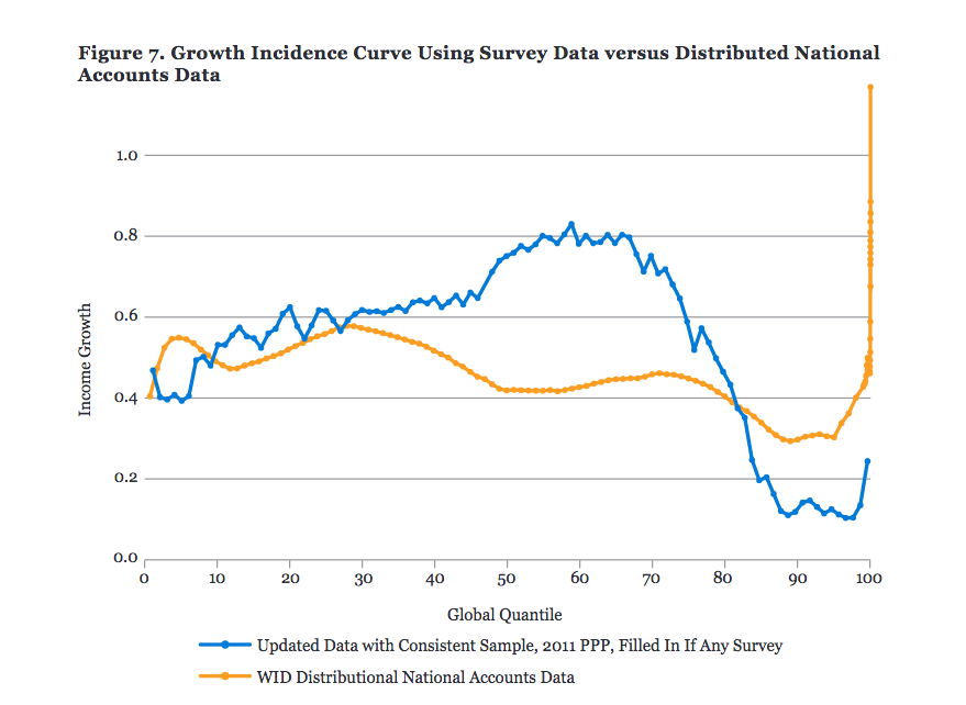
I include the graph with both data sources because Kharas & Seidel emphasize how each data source (surveys vs. tax records) has its own biases, and neither should be taken literally. Kharas & Seidel also discuss a number of possible methodological alterations that change how income growth graph looks.
Caveats aside, these data suggest that the world’s poorest decile experienced income growth at about the same rate as global economic growth, or maybe a little lower. This implies a q roughly between 0% and -0.5% based on Kharas & Seidel and World Bank data.
As I mentioned previously, most of the income growth in the past few decades among the world’s poorest happened in China and India, with sub-Saharan Africa getting left behind. Perhaps the global extreme poor will experience worse growth over the next 20-30 years now that the people in the rapidly-growing Asian countries have moved out of the bottom decile.
The aforementioned World Wealth and Income Database presents data on a wide variety of metrics. We can use their website to look at income growth for sub-Saharan Africa, the poorest region in the world, from 1980 to 2016. The whole region experienced an annual 0.9% increase in PPP-adjusted national income per capita, while the poorest 50% (which roughly corresponds to the bottom decile globally) saw 1.6% growth over the period. Or if we look at 1993-2013 to allow a direct comparison to the Kharas & Seidel data, we see 1.7% overall growth as well as 2.4% growth for the poorest 50%. These results suggest a historical q of around -0.5% to -1% for sub-Saharan Africa.
The past does not predict the future
In Capital in the Twenty-First Century6, Thomas Piketty presents some data on longer term trends on income growth going back about 200 years. These data cannot tell us much about extreme poverty because they only cover the most developed countries, but we can draw one key lesson. Income inequality increased from about 1870 to 1910, then decreased 1910 to 1950, and has been increasing again since then. This shows that income inequality can go through long periods of rising or falling, so the past 25 years in which we’ve had good global data probably don’t tell us much about what we can expect going forward.
That said, to my knowledge, the recent historical q of around 0% to -1% will plausibly continue over the next decades. Given the amount of research done in this area by development economists, we could probably develop a better estimate of q, but this level of inquiry suffices for now.
How quickly do giving opportunities disappear?
We discussed above why g + q determines the discount rate on cash transfers. We can always continue giving poor people money (at least in theory), so the best interventions must always be at least as good as cash transfers. Thismeans cash transfers get less cost-effective at the rate g + q.
But some interventions may do more good per dollar than direct cash transfers–such as the best global health interventions. (GiveWell thinks so.) In that case, even if cash transfers can absorb arbitrary amounts of funding, the better interventions might still dry up over time. If these better interventions do exist and they’ve been disappearing, that raises the question of why we don’t see this in global income statistics: why isn’t the bottom decile getting richer much faster than the global median?
There exist three possibilities:
- The best global health interventions do not actually do much more good than cash transfers.
- The best global health interventions increase people’s income more so than cash transfers, but they aren’t well-funded enough to show up in aggregate global income trends.
- Global health interventions do more good than cash transfers, but don’t produce a substantial increase in income.
In case 1, direct cash transfers do about as much good as anything else, so how much good we can do depends on how much poorer the poorest people are relative to us, the donors. In other words, giving opportunities dry up at about rate q.
Similarly, in case 2, the best giving opportunities are not being substantially funded, so giving opportunities will not disappear much quicker than the rate of income inequality reduction.
That leaves case 3, in which the best interventions actually do beat cash transfers, but don’t show up in q. In this case, top global health interventions will receive more and more funding over time10, until their cost-effectiveness converges with cash transfers’. How quickly this happens depends on (1) the current differential between cash transfers and the top intervention and (2) the time until convergence.
Based on GiveWell’s 2018 cost-effectiveness analysis, it’s reasonable to assume that the current best global health interventions are about 5 times more cost-effective than cash transfers11. If better-than-cash-transfer interventions take a given number of years to dry up, what marginal discount rate d should we apply on top of rate p?
| years | rate |
|---|---|
| 20 | 8.4% |
| 50 | 3.3% |
| 100 | 1.6% |
| 150 | 1.1% |
Or calculate for your own inputs:
(Clearly I don’t have great design skills but it gets the job done.)
Even over somewhat long time horizons (>50 years), this rate non-trivially increases the value of p. Even if giving later beats giving now for GiveDirectly, it is plausible that we should prefer to give now to GiveWell’s other top charities that have higher estimated cost-effectiveness.
By when should we expect the best interventions to converge with cash transfers?
I don’t have anything definitive to say about this, and more research would likely prove fruitful. That said, I have some observations, as follows.
- The industrial revolution began over 200 years ago, and we still have not come close to eradicating global poverty, so it would not be surprising if it took until 2100 or longer to end poverty.
- The number of people living in extreme poverty has roughly halved since 1990 (see Global Extreme Poverty by Our World in Data, which contains lots of well-presented data). That said:
- The international poverty line is an income of $1.90 per day. Someone making substantially more than that could still easily be considered poor.
- For a full picture of poverty, we should look at more than just income. The Global Extreme Poverty report above includes a section on multidimensional poverty. It would be a relatively straightforward matter to examine data on the multidimensional poverty index (or similar metrics) to better estimate how poverty has been changing over time.
- Effective giving opportunities may disappear more quickly than the poorest people’s lives get better, because there are many people living in poverty who nonetheless cannot easily be helped.
- Looking at specific metrics may overestimate the pace of poverty reduction. For Goodhart’s Law reasons, particular well-known indicators of well-being, such as child mortality rates, may show dramatic improvement over the course of a few decades while other unmeasured but important problems remain.
Could giving opportunities get better over time?
(In other words, could d be negative?) Perhaps in the future, we will discover new ways of doing good that work better than our current best efforts. That’s certainly conceivable. I don’t consider it a strong possibility, but I haven’t seriously considered the arguments in favor. I do believe we have a fair chance of improving on the current opportunities in smaller cause areas such as farm animal welfare, but global poverty is already well-funded and well-researched, so my best guess is that we have already found the best interventions.
Tentative Results
A probabilistic answer
A basic quantitative model would take point estimates for each of its inputs and produce a single answer. One could then adjust the point estimates to see a range of plausible answers.
For the problem under discussion, we can get a better picture by using a probabilistic model. Assume that each input follows a normal distribution (probably a reasonable simplifying assumption12), and provide a mean and standard deviation to define the distribution. Use these inputs to calculate probability distributions for r and p, and then calculate the probability that r > p, or the probability distribution of the difference r - p. If r - p > 0 that means the model says you should give later, and r - p < 0 means give now. Similarly, P(r > p) indicates the probability that giving later beats giving now.
(The math all works out nicely because the sum or difference of two normal distributions is itself a normal distribution where the mean is the sum or difference (respectively) of the two original distributions’ means.)
Estimation tool
I included some default values based on my rough best guesses at the time of this writing, but left the input fields blank to avoid anchoring. Feel free to change the inputs to fit your own best guesses. Press “Show defaults” to populate the inputs with my best guesses, and “Clear” to clear all inputs.
- Excluding alpha, I chose the values for
g + i + vto fit with Research Affiliates’ estimated 2.6% return and 1.7% standard deviation on projected 10-year world stock market returns (as of August 2018). - I arrived at alpha = 4% by taking the estimated 6% alpha from the cited sources in the section on alpha and adjusting for the expectation that alpha will be smaller in the future.
- In the section on q, I estimated that
qwas around 0% to -1%, so I chose -0.5% as the middle value with a standard deviation of 0.5%–one standard deviation in each direction covers my estimated range. This implies a 95% probability that the true value falls between -1.5% and 0.5%, which seems reasonable to me. d = 3.3%comes from the assumptions that (1) the best interventions are currently 5x better than cash transfers and (2) they will take about 50 years to converge.
Again, this model does not give the true probability that giving later does more good than giving now. The model only considers the investment rate and the donation discount rate. We can and should consider lots of other factors that weigh into the decision.
If global inequality is rising, that might mean you should donate later
Rising income inequality generally is considered a bad thing because it works to the disadvantage of the world’s poorest people. But somewhat counterintuitively, the greater the disparity in income growth, the more likely it is that we should not do anything about it, because we can do more good by waiting until income inequality gets worse.
This is not to say that we necessarily should give later if inequality is rising; but the smaller the value of q, the more the balance tips toward giving later.
The conclusion depends on α, which defies attempts to learn its value
We can estimate the historical value of alpha as I did above. But markets are anti-inductive. Market anomalies tend to disappear over time, which makes it harder to outperform a broad index.
As discussed above, we do have some reason to expect certain market inefficiencies to persist. They probably will not work as well in the future as they did in the past, but how less well will they work? Half as well? A quarter as well?
The value premium has been well publicized at least since Ben Graham and David Dodd’s Security Analysis in 1934 and Graham’s The Intelligent Investor in 1949. But value investing has become much more popular in recent years, as seen in the growth of value mutual funds and smart beta funds. On the other hand, some evidence suggests that investors are not harvesting the value premium in general. For example, David Blitz’s Are Exchange-Traded Funds Harvesting Factor Premiums? found that for every dollar in a value ETF, there’s (approximately) one dollar in an ETF following the opposite strategy.
It’s plausible that the value premium (and perhaps other sources of alpha) will work just as well in the coming decades as they have in the past. And perhaps they will work far less well. I have no idea.
Should we disprefer investing in risky assets?
None of the prior discussion considered the nature of risk in investing. Nearly all investors don’t just care about their expected return, but also their risk. What should we care about?
If we invest to give later, we introduce the possibility that we will lose money on our investments, and end up donating less than if we had given now.
Altruists should generally not be as risk-averse as people investing their personal money, so we can largely ignore investment risk without losing much. That said, there is certainly room for further analysis on this. Considering risk would make giving later look relatively worse, but it’s hard to say by how much.
What if you use leverage?
If you’re investing your money to donate, you might be willing to pursue more risky investments than you would otherwise. For this essay, I have assumed that you invest entirely in stocks and not bonds, which already has greater risk than investors usually take on. But you can take on even more risk via leverage: borrow extra money so that you can invest it. You may be able to substantially increase r by taking on leverage.
This naturally raises the question of how much leverage you should use. Brian Tomasik discusses this in some detail. It’s a complicated question, and unfortunately, it introduces a huge amount of uncertainty into what return on investment you might expect.
Suppose instead of holding stocks with no leverage, we used 2:1 leverage. This would somewhat less than double our expected return. (Tomasik has extensive calculations and simulations on what return we might expect.) For simplicity, let’s coarsely assume that we make 1.5x greater return by using 2:1 leverage. If we previously used r = 4%, now we have r = 6%, which could easily tip the balance from donating to saving. If we previously used a more aggressive r = 8%, leverage jumps our return up to 12%, which pushes strongly in the direction of giving later.
Extra Details
There is much to consider about the investment rate vs. the discount rate, so I have tried to focus only on the most relevant details. One could add many caveats, complications, and additional assumptions to my analysis up to this point. In this part, I will address what I see as some of the most important ancillary considerations.
Qualitative factors may tilt the scales toward giving now
Julia Wise’s Giving Now vs. Later: A Summary lists some commonly cited arguments in each direction. My essay’s model incorporates most of the arguments for giving later, but doesn’t cover several of the arguments for giving now.
Julia’s reasons to give now:
You may get less altruistic as you age, so if you wait you may never actually donate. Estimates of the returns on investment may be over-optimistic. Giving to charities that can demonstrate their effectiveness provides an incentive for charities to get better at demonstrating that they’re effective. We can’t just wait for charities to improve — it takes donations to make that happen. Having an active culture of giving encourages other people to give, too. Better to eliminate problems as soon as possible. E.g. if we had eliminated smallpox in 1967 instead of 1977, many people would have been spared.
Julia’s reasons to give later:
As time passes, we’ll probably have better information about which interventions work best. Even in a few years, we may know a lot more than we do now and be able to give to better causes. Investing money may yield more money to eventually donate. When you’re young, you should invest in developing yourself and your career, which will let you help more later. You can put donations in a donor-advised fund to ensure they will someday be given, even if you haven’t yet figured out where you want them to go.
Naturally, the importance of each of these considerations is a matter of debate; but the model does seem somewhat biased in favor of giving later because it does a worse job of accounting for the considerations for giving now.
There are three main ways of giving later, all of which have problems
If you want to save your money to donate later, you essentially have three options for how to store it:
- Keep your money in a taxable account.
- Give it to a donor-advised fund (DAF).
- Set up a foundation.
The first option offers the most flexibility, but it has one big problem: taxes. You can deduct donations from your income up to a certain limit (in the United States, you can deduct up to 30% of your income if you’re donating appreciated assets). If you donate a lot of money all at once instead of donating every year, you will likely hit the deduction limit and won’t get any tax savings on most of your donation.
You can solve this by giving your money to a donor-advised fund. A DAF is a charity (usually a subsidiary of a brokerage firm like Fidelity or Schwab) that invests your money and can make grants based on your recommendations. You can continue investing your money once it’s in a DAF, but because the DAF is itself a charity, contributions are deductible.
The third option: set up a foundation to hold your money. This has high startup and overhead costs–it’s no coincidence that usually only high net worth people start foundations. In addition, foundations are legally required to disburse at least 5% of their funds per year, so this option isn’t so much “give later” as it is “give a little bit every year and then a lump sum later if you even have any left.”
Investing looks particularly bad right now, but only under certain assumptions
Countries’ stock market returns in the long run have tended to cluster around 5%. Unfortunately, the market outlook today looks worse. Due to relatively low yields and high valuations, Research Affiliates projects a 2.6% 10-year real return on the global stock market (as of August 2018). The projection for the US market looks even worse, at 0.2%. This may point in favor of donating now, at least until return expectations improve–although not necessarily, as discussed in a different section.
Note that the substandard global market outlook largely comes from the United States’ current high valuation, because the US currently accounts for about half the global market capitalization. Research Affiliates projects a relatively normal 5% return for global stocks excluding the US.
Research Affiliates’ projections include three components: capital growth, net yield, and valuation. An efficient-markets hardliner would exclude the valuation component of these projections; doing so shifts the expected global return from 2.6% to 3.8% and the US return from 0.2% up to 3.1%.
If you do believe valuation estimates tell us something useful, you can outperform the global market in expectation by seeking undervalued segments. Research Affiliates estimates a 6.8% average 10-year return for emerging markets due to low valuations. Or one could go even further with something like GVAL, an ETF that buys stocks in the 25% cheapest out of the 45-ish countries that have investable public markets. Your estimate for projected future return can vary greatly based on which of these assumptions you make.
Should you give later if you expect investment returns to improve?
If you expect investment returns in the near future to underperform the donation discount rate but to improve in the future, you may prefer to save your money even though donating looks better in the short term. Consider an example. For simplicity, let’s say the discount rate p is 2%, and the expected investment return r is a flat 0% for the next year. But the year after that, r will jump up to 10%. Suppose you donate $1 per year.
If you donate your money at the beginning of this year, you will donate a total of $1 (obviously). If you wait a year to donate, your discounted donation will only be worth $0.98 in today’s dollars–a 0% investment return combined with a 2% discount. So for a one-year time horizon, donating now wins.
If instead you wait two years and let the money keep compounding, the situation changes. The naive strategy is to donate immediately whenever p > r and save your money when r > p. Under our example, that means you donate at the beginning of the first year, and then for the second year you invest your money and donate at the end. The naive strategy results in a total present-value donation of $2.06 (a first donation worth $1, and a second donation that’s discounted at 2% for two years and earns 10% return for one year).
However, if you wait two years before donating anything, the present value of your donation will reach $2.11. Your donation is worth more in this case because even though your first dollar loses an extra 2% due to time discounting, you make up for it by earning 10% return in the second year.
The takeaway: if you expect to earn a subpar return for some years but expect the return to increase, such that your average investment return will exceed the discount rate, you are better off waiting. This requires both that the investment return will increase and that you have a sufficiently long time horizon to take advantage of it. This has relevance for investors today given that the market will probably have a better average return over the next 30 years than over the next 10.
Note that we cannot make the same argument in the opposite direction. If you expect investment returns to get worse at some point in the future, you should simply save your money until r crosses below p, at which time you should donate all your savings.
What if donations produce compounding returns?
As argued by Holden in 200713:
[Y]ou get a much higher ‘return’ on charity than you get on investing. Both companies and the poor can create more value if you give them more money; the difference is that investing, where the value accrues to you, is way more popular than giving, where it doesn’t. Therefore, giving is ‘cheaper,’ and your expenditures today multiply more.
Some have argued that well-directed donations will compound at a faster rate than investments. Paul Christiano responds:
Here’s the problem: if you give your money well, it might compound much faster than it would have in your bank account—but only for a while. Over time the positive effects will spread out more and more, across a broader and broader group of beneficiaries, until eventually you are just contributing to a representative basket of all human activities. Eventually, my investment will compound at the rate of world economic growth, rather than at the particularly promising interest rate I was able to originally identify.
When I leave money in my bank account, it compounds slightly (1-2%, conservatively) faster than world economic growth. It does this for years, until I decide to spend it, for example on developing world aid. At that point it will earn anomalously high returns for a while, before being spread out throughout the world and then compounding in line with world economic growth. If I donate a year later, I earn 1 extra year of market returns, and 1 less year of compounding in line with economic growth. That’s a good deal—an extra 1-2%.
[…]
So if I’m considering donating to a cause like developing world aid, I shouldn’t donate sooner rather than later just because poor folks can earn higher returns than I can. I should instead look at the total multiplier I’m getting on my money, and donate if and only if I expect that multiplier is declining faster than [(market rates of return) – (economic growth)]. I don’t think we’ve found many causes for which this is plausibly the case, and I think that aid is definitely not one of them.
As Christiano says, we only care about the compounding rate of donations if we expect that rate to decline in the future. We can think of the extra compounding as part of the value of the donation: when we donate, we produce some immediate value, plus some extra value due to compounding that eventually runs out. Sum up the total value produced (factoring in time discounting) and call that the value of your donation.
For example, suppose donation A will produce $100 worth of value immediately but no compounding effects. Donation B will produce $30 of value immediately and produce compounding benefits over time, and by the time the compounding reverts to the base level growth rate, it will have produced $70 of time-discounted value. You can consider donations A and B equivalent, which means you don’t actually care if a donation has compounding effects for the purposes of giving now vs. later; all you care about is the total magnitude.
It matters if the compounding portion of a donation made now has a bigger impact than the compounding portion of a donation made later:
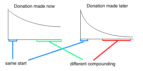
We should be able to roughly account for this when looking at how global development opportunities will change in general; I don’t believe it requires any special consideration. Simply consider the value of the donation as the whole area under the curve.
Existential risk makes giving later look worse
If civilization has a nontrivial probability of irrecoverably collapsing in the next century, that puts a blight on potential good done later. (You can’t help the global poor if everyone is dead.) You can account for this by discounting future donations by the annual probability of global catastrophe/extinction. The calculator I wrote does not offer an input for this, but you can account for existential risk (x-risk) by increasing the mean and standard deviation of d based on your estimated annual probability of extinction and confidence in your estimate.
I was unsure whether to consider this a central or ancillary concern. If you believe x-risk has a nontrivial probability, you might prefer to donate to x-risk prevention efforts rather than global poverty. On the other hand, you may believe x-risks are non-negligible but not know of any tractable solutions, and thus prefer to donate to global poverty. In that case, it would be reasonable to care about the discount rate on global poverty but also apply a discount based on the probability of extinction.
That said, bringing up existential risk raises other complicating considerations. A global catastrophe that falls short of extinction might actually make future donations look better than present donations. For example, climate change could make things much worse for poor people living in the most affected regions of the world, while you personally might remain insulated from the effects. Your donations will go further in this future world than they will today. So you might want to add a premium rather than a discount on future donations.
Given the complexity of these considerations, I left them out of the main portion of the essay; but some readers may wish to take them into account.
If the best global health interventions are getting used up (a.k.a. d > 0), why hasn’t the bottom decile experienced greater income growth?
I don’t really understand this. We could reach a couple of possible explanations:
- Maybe there aren’t very many really good health interventions–only a small percent of the global poor can be helped more cheaply than cash transfers–so the benefits they provide don’t show up in aggregate statistics.
- Maybe the best health interventions improve people’s lives without affecting their income growth.
The first explanation seems unlikely because health outcomes for the global poor have improved dramatically since 1998 (and in 1998 they had improved equally dramatically over 1978). If the global poor are getting healthier, you would expect to find lots of opportunities to help them get healthier even faster.
The second explanation would be somewhat surprising if true–improving people’s health outcomes should help them achieve their goals better, which should translate into higher income.
I don’t find either of these explanations satisfying. Perhaps they’re both partially true. Perhaps there’s some dominant third factor that I haven’t thought of. I do not consider this question hugely important to this essay, but it’s a related puzzle. Perhaps someone who knows more than I do about global development can answer it.
Concluding Remarks
When I began writing this essay, I initially expected to find that giving now looked better than giving later. But according to this model, using my best estimates of the input variables, giving later beats giving now with unexpectedly high probability. That said, some qualitative factors not accounted for by the model push toward giving now. And of course, for cause areas other than global poverty, the analysis would look quite different.
The main takeaway should be not so much an answer to the now vs. later question as a general approach. Namely, it is possible to break down the investment rate and discount rate to get a more accurate answer, as well as a sense of how that answer varies with different inputs. Robin Hanson’s claim–that r > g and therefore we should give later–provides a reasonable starting point, and we can get a much better picture by examining the factors that influence the investment rate and discount rate. This analysis certainly doesn’t include every important consideration, but I hope it can add some clarity to the question of giving now vs. later for global poverty interventions.
Thanks to Linda Neavel Dickens and Jake McKinnon for reviewing drafts of this essay.
Notes
-
In practice it’s hard to ensure that your money gets put to good use long after you’re dead. For more on this, see Hanson, Let Us Give To Future. ↩
-
Strictly speaking,
idoesn’t have to grow with GDP. Companies may choose to use some or all of their free cash flow to pay out dividends, soidepends on what portion of free cash flow companies return to shareholders, as well as what portion of GDP ends up as corporate free cash flow. These portions may fluctuate somewhat over time, but they should stay within a fairly narrow range; and in the long run the ratio of shareholder yield to GDP should remain stable. ↩ -
GiveWell’s 2018 cost-effectiveness analysis assumes that utility is logarithmic with consumption. (Note that consumption and income can be considered roughly the same thing for our purposes.) See also: Betsey Stevenson & Justin Wolfers (2013), “Subjective Well-Being and Income: Is There Any Evidence of Satiation?” National Bureau of Economic Research. ↩
-
Homi Kharas & Brina Seidel (2018). “What’s Happening to the World Income Distribution?: The Elephant Chart Revisited”. Brookings Institution. ↩ ↩2
-
Meb Faber (2015). Global Asset Allocation. Downloadable for free at https://mebfaber.com/books/ as of this writing. ↩ ↩2
-
Thomas Piketty (2013). Capital in the Twenty-First Century. ISBN 978-0674430006. ↩ ↩2
-
Wesley Gray, Jack Vogel, and David Foulke (2015). DIY Financial Advisor. ISBN 978-1119071501. See also The Value Momentum Trend Philosophy, a blog post by Wesley Gray on similar topics. ↩
-
Income inequality sometimes refers to the differential between the richest and the poorest people. But for our purposes, that’s not an important comparison because we use the investment rate of return as a more precise estimate of what rich people (a.k.a. we) can earn. So I define income inequality as the relative difference between the poorest people and the global average. ↩
-
This is specifically for recipients in Kenya. ↩
-
Assuming there are sufficiently many effectiveness-minded donors, which appears to be the case, large donors such as government aid programs and major foundations currently do a reasonable job of identifying and funding the best global health interventions. ↩
-
Methodology: GiveWell presents cost-effectiveness estimates from 11 different GiveWell researchers and then takes the median for each charity. I then took the median of all the charities’ medians, excluding GiveDirectly (because that’s the baseline we are comparing to) and Against Malaria Foundation/Malaria Consortium (to avoid concerns about population ethics). Including the malaria charities changes the median from 5.1 to 5.3. ↩
-
What if input parameter values are not normally distributed? Possibly, the parameters have fatter-than-normal distributions or they’re skewed rather than symmetric. If parameters have fat-tailed distributions, that does not decrease the certainty of the model result, but it does increase the probability that the
|r - p|spread is large.
If any parameters have skewed distributions, that could affect the outcome in a variety of hard-to-predict ways. More generally, if we move away from normal distributions, we need the model to specify much more information about the shape of the distribution for each parameter. I believe this provides little value given the effort required, so I have stuck with the assumption that all inputs follow normal distributions. ↩ -
I do not know whether Holden today still endorses his 2007 belief. ↩