Reading Notes
Preamble
This page contains my reading notes on most important articles I've read since 2015. I take notes on articles I want to remember.
You can click on a tag to show only notes with that tag, and click the tag again to show all notes.
Most of the time, first-person pronouns in my notes refer to the author of the book/article, not to me. Lines preceded by "me:" give my own thoughts.
Disclaimers:
- I primarily write these notes for my own benefit, so some parts might not make sense. But I hope you find something useful in them.
- Unless otherwise specified, these notes represent my interpretation of the authors' views, not my own views. But also I can't promise that I understood the authors' views correctly.
- I exported my notes from org-mode to HTML with minimal editing. Some things might not look right.
Readings
Dynomight: My advice on (internet) writing, for what it's worth
https://dynomight.net/writing-advice/
- Make something you would actually like
- Nobody really understands anyone else. You can't predict exactly what other people would like. But you can predict what YOU like
- My blog is weird because I like weird
- But your brain is lying to you. If someone else wrote your post, would you actually like it?
- If you run out of ideas, just take one of your old ones and do it again, better. It's fine, I promise
- Editing exercise: Go through and circle the good parts. Then delete everything else
- Be funny, maybe. You fuckers all take yourselves too seriously
- But humor needs to be worth it (short jokes are cheaper than long jokes)
- Write for your allies, not your haters
- Clear writing is next to godliness. But the optimal number of confused readers is not zero
- Some writers get bogged down in doing new research. But if you already believe something, then either you have good reasons, or you don't. Just explain why you believe it
Some things I noticed while LARPing as a grantmaker causepri
(abridged notes)
- You should probably be like I do research to figure out what projects should exist, then make them exist rather than I evaluate the applications that come to me
- Winner's curse: If you're more excited about X than your peers, that's evidence that X is not as good as you think
- Fear theories of change that route through "empower this sketchy person and hope they do good things"
- me: There's a conflict between winner's curse and the neglectedness heuristic
- Perhaps an important discriminator is: Can you identify a reason why others under-rate this intervention?
Willingness to look stupid is a genuine moat in creative work self_optimization
https://sharif.io/looking-stupid
- Richard Hamming: Nobel Prize winners stop doing great work after they win the prize because they're trying to find the next big thing, instead of planting the little acorns from which mighty oak trees grow
- Many good ideas come from young and unproven people. I don't think young people are smarter than old people, or work that much harder; but they're not afraid of looking stupid
- HN: Young people do worry about looking stupid, they just don't know that they look stupid
- We wanted to write something clever on a birthday cake. We decided "Let's say a bunch of ideas out loud so we can get to the good ones." And it worked!
- Evolution lets mutations get locally worse, and sometimes they get globally better. If evolution had a sense of shame, it wouldn't work
- The trick is don't try to share something good. That's a game you can lose, and you won't want to lose. Instead, play the game of sharing something at all
Rational Reminder: Should gold and other metals be considered in portfolio allocation? finance
summary of best comments from https://community.rationalreminder.ca/t/should-gold-and-other-metals-be-considered-in-portfolio-allocation/13250
- Gold has worked as an inflation hedge over multi-century time horizons. Gold in Ancient Rome could buy a similar amount of goods as gold today. But gold is not a good inflation hedge even over 50-year horizons
- Golds are not a replacement for bonds. The defining characteristic of Treasury bonds is that they provide predictable cashflows (or even real cashflows if you buy TIPS). Gold's price is volatile and there is no strong reason to expect positive real returns
- 1975–2001 gold declined 60% after inflation. "A good store of value does not have 60% losses in purchasing power over long-term investment horizons"
- Jastram (1977): Over 400 years of history, gold made for a poor inflation hedge. During inflationary periods between 1933 and 1967, gold performed worse than a commodity index
- Erb & Harvey (2013): "While gold might protect against inflation in the very long run, 10 years is not the long run. In the shorter run, gold is a volatile investment which is capable and likely to overshoot or undershoot any notion of fair value."
- They found that gold exhibits some mean reversion when it is above or below the long-run average real price
- F&F: Owners of gold jewelry earn a "consumption dividend" (i.e. they benefit from using the gold as well as owning it). If gold is correctly priced, then investors who don't earn the consumption dividend should prefer not to hold gold
- People make the mistake of comparing the historical 0.7–1% real return on gold to the present-day [as of 2021] <1% yield on bonds. But gold doesn't look so good when you notice that bonds had a long-run real yield of 1.6%
- If you take an asset with completely random returns and replace some of your equities with it, and look at the portfolio during the worst period for equities, it will necessarily look better than the 100%-equities portfolio
- In the UK, gold had >50% real drawdowns 1562–1592, 1738–1801, and 1897–1920 (source: The Golden Constant (book))
Quantica: Are Trendfollowing CTAs Truly Long Volatility? (2023) finance trend
https://quantica-capital.com/publications//pdf/2023Q4_QuanticaQuarterlyInsights.pdf
see also FrankieC's backtests
- 2000–2023, trend performed well when VIX was low, medium, or high, but returns came from different sources
- low VIX: high equity trend return; ~zero return from other assets
- med VIX: ~equal returns from all assets
- high VIX: dominated by fixed income
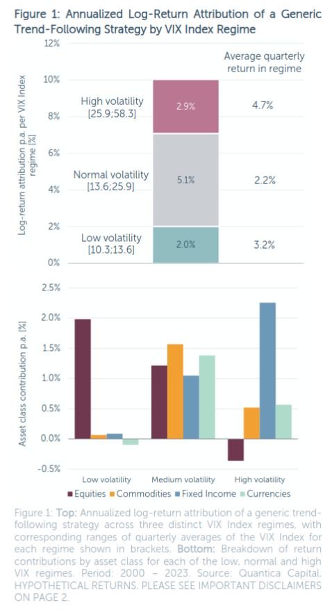
- me: I replicated this finding out of sample (1990–1999) and found that med-VIX and high-VIX looked similar to in-sample, but low-VIX did not show returns being dominated by equities
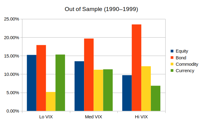
- When looking at realized volatility for each individual asset class:
- Trend (aggregate) had positive returns in all three regimes
- Trend (aggregate) performed best when that asset had low vol
- In low-vol regimes, equities did best and commodities/currencies did worst for each asset class
- In med-vol regimes, asset class returns were fairly balanced
- In high-vol regimes, bonds did best and equities did worst for each asset class
- when bond vol was high, bonds still did best
- High-vol regimes across asset classes had less than 50% overlap
- me: bonds had stronger uptrends in high-VIX regimes, while equities (unsurprisingly) had downtrends
Methodology
- Our trendfollowing strategy uses medium-to-long-term trends, designed to track the SG Trend Index
- Universe includes 20 equity markets (16 countries), 17 bonds, 8 currencies, 16 commodities
- We define, low, medium, and high vol as bottom 16%, middle 68%, and top 16%
- Look at (non-overlapping) quarterly returns 2000–2023
Cam Harvey: Presidential Address – The Scientific Outlook in Financial Economics (2016) finance stats
https://people.duke.edu/~charvey/Research/Published_Papers/P131_The_scientific_outlook.pdf
- Minimum Bayes Factor (MBF) is the odds ratio under the assumption that if the null hypothesis is false, then the true value exactly equals the mean in the observed data
- me: This is the reciprocal of the likelihood ratio as I've been using it
- If we don't have a fixed prior but we think the prior distribution should be symmetric and descending around the null, then we can calculate the symmetric and descending MBF (or SD-MBF) as
–exp(1) * p-value * log(p-value)- ex: for a p-value of 0.05 on a normal distribution, MBF = 0.147; SD-MBF = 0.407
- Multiply MBF by the prior odds of the null to get the posterior odds of the null;
probability = odds / (1 + odds)
Rational Reminder: The "AI Bubble" and Stock Market Concentration finance
- Historically, high valuations predicted poor future returns, but high market concentration didn't
- 20: It's not just that the US market is concentrated, it's that the biggest companies are also in similar lines of business
- Chart @49min shows Switzerland having the most concentrated market in 2015, but the top 7 companies were diversified across 5 sectors
- plus the largest developed-market company is ASML and the largest emerging-market company is TSMC
- 38: Around 2000, the US market fairly quickly switched from net issuing stock to net buying back stock. D/P as a predictor of market returns is misleading, but if you look at D/P plus 10-year cyclically-adjusted buybacks, current US market expectations look about average
- 113: Attempted to replicate #38 for Japan but the data doesn't go back far enough. Japan and Europe have continued to net issue shares
- 124: I wish the podcast had talked about whether they actually think we're in an AI bubble
- 142: The podcast didn't take a stance on whether we're in an AI bubble because they think it's better not to try to predict bubbles, and have a diversified portfolio that's prepared for both bubbles and crashes
- 167: Perhaps the reason why bonds look so abysmal in the Cederburg data is that stocks are indeed better than bonds for most households, but households are not the average investor: a huge % of investors are intermediaries with strict capital requirements, which creates demand for bonds
- 265: DFA: current market is not like 1999 because profitability growth is higher: profitability increased 2021–2025 whereas it decreased 1995–1999
AQR: A Century of Evidence on Trend-Following Investing (2017) finance trend
https://www.aqr.com/Insights/Research/Journal-Article/A-Century-of-Evidence-on-Trend-Following-Investing PDF see also [2018-10-04] AQR: A Century of Evidence on Trend-Following Investing (2017) (old) but I believe those notes are based on an old draft because the contents don't match. notably, gross/net returns changed from 14.9/11.2 to 18.0/7.3
Introduction
- Was the good performance of trendfollowing 1985–2015 a fluke, or a long-term phenomenon?
- We construct TSMOM data going back to 1880
- We use monthly returns for 67 markets: 29 commodity futures, 11 equity indices, 15 bond markets, and 12 currency pairs
- We construct an equal-weighted combination of 1-month, 3-month, and 12-month TSMOM strategies. Go long or short based on positive/negative excess return, vol-weight positions, and target an ex ante 10% vol (weightings go down when ex-ante correlations go up)
Performance (1880–2016)
| gross excess return | 18.0 |
| net of costs | 11.0 |
| net of costs + 2/20 fee | 7.3 |
| volatility | 9.7 |
| Sharpe net of fees+costs | 0.76 |
| correlation (US equities) | -0.01 |
| correlation (US 10Y) | -0.03 |
- Positive net Sharpe ratio in every decade
- Lowest-return as well as highest-stdev and lowest-Sharpe decade was 1910-1919; second-worst decade was 1880–1899. 2010–2016 was third-worst
Performance by trend signal
- gross of costs and fees
- "lagged" = signal is lagged by one month: trend signal is computed at EOM January, but not traded until EOM February
| Signal | Sharpe | Sharpe (lagged) |
|---|---|---|
| 1-month | 1.38 | 0.45 |
| 3-month | 1.19 | 0.65 |
| 12-month | 1.32 | 1.04 |
Performance during crisis periods
- "Trend smile": TSMOM has done particularly well in extreme up or down years
- During the 10 worst drawdowns for US 60/40, TSMOM had positive returns in 8 out of 10 drawdowns (gross of fee, net of cost). Only exceptions are 1937 recession and 1987 crash where TSMOM was slightly negative
- Average of those drawdowns lasted 15 months from peak to trough
Performance across economic environments
annualized excess return (t-stat) Sharpe ratio
| Group 1 | Group 2 | Difference | |
|---|---|---|---|
| recession vs. boom | 10.4% (5.4) | 11.2% (10.7) | 0.8% (0.4) |
| low vs. hi inflation | 10.5% (8.4) | 11.5% (8.4) | 1.0% (0.5) |
| stocks: bull vs. bear | 10.2% (10.4) | 15.5% (5.9) | 5.3% (1.9) |
- me: volatilities were also reported, but hardly varied across regimes
- Dividing S&P volatility (36-mo) into quintiles, trend performed much better in quintiles 2 and 3
Appendix B: Simulation of transaction costs
- We estimated post-2002 costs from AQR's trading data
- We assumed costs were 2x as high 1993–2002 and 6x as high 1880–1992, based on Jones, C. M. (2002). A Century of Stock Market Liquidity and Trading Costs.
One-way transaction costs:
| 1880–1992 | 1993–2002 | 2003–2016 | |
|---|---|---|---|
| equity indices | 0.34% | 0.11% | 0.06% |
| bonds | 0.06% | 0.02% | 0.01% |
| commodities | 0.58% | 0.19% | 0.10% |
| currencies | 0.18% | 0.06% | 0.03% |
me: remember that 10% vol TSMOM has maybe 400% net leverage. for a modern fund that's 0.40% per 100% turnover, and 0.80% to go from full long to full short
Avantis: Our Scientific Approach to Investing finance factors funds
Valuation lays the foundation
- We look for stocks with higher implied discount rates (= high expected returns)
- me: I doubt that value/profitability premia are explained by varying discount rates across securities. Speculators can buy any security but they only have one discount rate
- Valuation equation: Price = Book Value + Profits / Discount Rate
- Two ratios to determine relative value: Book/Price and Earnings/Book
- High B/P means a company either has low profitability or high discount rate, but we don't know which. High B/P and high profitability means a high discount rate
- me: I don't get why you don't just use E/P or CF/P. Top 30% value portfolios have the following RMW loadings on a Beta + RMW regression: B/M = –0.12, E/P = 0.17, CF/P = 0.19
Profitability
- Novy-Marx (2013) discovered that gross profit is a better measure than earnings because it excludes more non-recurring and discretionary items
- Gross profit minus selling, general, and administrative expenses gives operating profit; OP is better for comparing across sectors because some sectors assign expenses through SG&A instead of COGS. We also subtract interest expense to penalize leverage
- Ray Ball (2016): Operating profits minus accruals (= cash profitability) leads to more predictable future profits. OP t-stat 3.65; cash profitability t-stat 6.29
Adjusted book-to-market
- Accounting definition of book value changed in 2000. Goodwill includes the amount an acquiring company pays for an acquisition beyond the book value, representing the acquisition's discounted cash flows
- This should not be considered equity any more than the acquirer's future cash flows are
- The more overpriced an acquisition is, the more it increases the book value of the acquirer
- B/M favors companies that do a lot of M&A, which historically have worse returns. Subtracting goodwill fixes this
- In 2019, goodwill accounted for 40% of aggregate book equity in the US
Value and profitability — stronger together
- We weight companies by market cap and then overweight or underweight based on their ranking on our joint value + profitability measurement
Incorporating additional information
Investment
- The intuition is that companies reinvest when discount rates are low, causing subsequent underperformance
- We exclude companies with high investment that don't look good on value + profitability
- me: They were not clear about how much weight they assign to the investment factor
Momentum
- Momentum is a strong factor but it requires frequent trading
- We use two measures of momentum
- Delay purchase of stocks with weak 6-month momentum and delay sale of stocks with strong 6-month momentum
- Lag price by 3 months in B/M (similar to HML factor) to avoid buying value stocks that are only cheap because the price dropped recently, and similarly when selling
- me: unclear whether they use both up-to-date B/M and lagged B/M, or exclusively lagged B/M
Trading — don't put all your eggs in one basket
- Turnover timing matters. Don't put all your trades for the year on the same day
- We rebalance daily, but only a little bit each day
Two Centuries of Multi-Asset Momentum (2017) momentum finance
https://papers.ssrn.com/sol3/papers.cfm?abstract_id=2607730
- Pairwise correlations in momentum portfolios have increased recently
Momentum over the long run
- Seven momentum strategies:
- country equity indices
- currencies
- government bonds
- commodities
- country-neutral sectors
- US stocks
- cross-asset-class
- combined
- Momentum is defined as top 1/3 minus bottom 1/3 by 10-month return, skipping most recent two months. Equal-weighted across assets
Tables
Table II: Global multi-asset momentum
monthly total returns (abridged). t-stats are for long/short
| long/short | long-only | t-stat | |
|---|---|---|---|
| equity indices (local) | 0.66% | 0.35% | 7.5 |
| equity indices (USD) | 0.63% | 0.28% | 5.7 |
| US stocks | 0.81% | 0.40% | 6.7 |
| cross-asset | 0.66% | 0.33% | 12.1 |
| combined | 0.40% | 0.20% | 14.0 |
GDP-weighted (Table XIV) and volatility-weighted (XV) are pretty similar
Table III: Momentum by decade
- me: about 1/4 of decades had negative returns; but Global Sectors, Cross-Asset, and Combined were almost always positive
Table VI: Reversal (skip months)
- me: short-term reversals in US stocks were so strong that "10-month no skip" momentum had a negative return
Table VIII: Momentum correlations
- Average pairwise correlation
- Full history: 0.11
- 2009–2014: 0.43
Table XVI: Global multi-asset class trend
10-month trend (no skip). monthly total returns (abridged). t-stats are for long/short
| long/short | long-only | t-stat | |
|---|---|---|---|
| equity indices (local) | 0.28% | 0.10% | 2.7 |
| US stocks | 0.68% | 0.20% | 6.8 |
| cross-asset | 0.66% | 0.17% | 13.2 |
| combined | 0.18% | 0.07% | 7.9 |
0.63 correlation to momentum
AGIX whitepaper finance ai
- lot of marketing BS
- "AI is not only a new technology layer, but it is a labor and GDP multiplier." good, they get it
- "As employees orchestrate 5–10 software agents that write code" that's not how LLMs work but the implication is correct that there are effectively way more workers
- stock selection is done by a team of "experts" including external advisors. quality of the fund comes down to whether those experts know what they're doing, but it's not transparent who their experts are, so it's hard to have confidence
Factor Momentum and the Momentum Factor (2021) momentum finance
https://papers.ssrn.com/sol3/papers.cfm?abstract_id=3014521 PDF
- Stock momentum is explained by factor momentum
- The average factor earns a monthly return of 6 bps following a negative year and 51 bps following a positive year
- Factor momentum subsumes stock momentum
- Momentum is not a distinct factor; it times other factors
Introduction
- Among 20 factors, the average factor earns a monthly return of 6 bps following a negative year and 51 bps following a positive year (t = 4.22)
- Factor trend earns an annualized return of 3.9% (t = 7.01)
- Factor autocorrelation may be explained by persistence of investor sentiment + arbitrageurs not wanting to expose themselves to factor risk
- We run PCA on 47 factors. We find that factor momentum concentrates in the high-eigenvalue principal components, that is, in factors that explain more of the cross section of returns
- A momentum strategy on the top 10 principal components has five-factor alpha with t = 6.51
- me: the FF five-factor model doesn't include momentum
- This finding is consistent with limits to arbitrage. If low-eigenvalue factors exhibited momentum, arbitrageurs could profit without assuming much factor risk
- A momentum strategy on the top 10 principal components has five-factor alpha with t = 6.51
- Figure 1: We test 6 different implementations of stock momentum
- Regressed on FF5, they all have alphas with strong t-stats
- Regressed on FF5 + factor momentum, they all have near-zero t-stats
- me: this is for real, not frequentist BS. standard momentum, industry momentum, and Sharpe momentum all have negative alpha; three other versions of momentum have positive but really weak alphas
- Regressed on FF5 + stock momentum, factor momentum has t = 5.32; regressed on FF5 alone, t = 7.53
- Factor momentum explains why momentum stocks are correlated with each other: they comove because they are exposed to the same factors
Wes Gray on factor momentum subsuming stock momentum
https://www.youtube.com/watch?v=uDhvHEPZgac
- There are other papers that do simpler versions of factor momentum and find that it doesn't have explanatory power
- There's contradictory research and it's unclear
- Intuitively, momentum is a greed trade. People see stocks going up and buy them. Momentum front-runs those people
- For factor momentum, I can't think of a story that I can write on a napkin
- Stock momentum and factor momentum probably get you to the same place but I'm more comfortable at an intuitive level with stock momentum
Quick notes on contradictory evidence
- me: This is a good reminder of why you should wait for replications before pursuing a new strategy. A paper can come up with really solid results, but then more papers come out and it starts to look less solid
Factor momentum versus price momentum: Insights from international markets (2024)
- Factor momentum is strong internationally, but its ability to explain stock momentum depends on methodological and dataset choices
- Stock momentum often better explains factor momentum than vice versa
- Specifically, PCA-based factor momentum explains stock momentum better than standard factor momentum does
The Many Facets of Stock Momentum: Distinguishing Factor and Stock Components (2025)
see also AlphaArchitect summary
- There is a stock-specific component of momentum tied to earnings news that isn't explained by factor momentum
GMO: Risk and Premium – A Tale of Value (2019) finance value
https://www.gmo.com/americas/research-library/risk-and-premium-a-tale-of-value_whitepaper/
- When decomposing value factor returns, we find that the recent poor performance is equally attributed to a reduction in the value premium and a widening of the value spread
- Value might deserve to trade at a deeper discount due to current market dynamics, but we believe value will still deliver a premium
- me: This article is better than the Research Affiliates one; it goes into value's reduced structural return
Introduction
- Possible explanations for value's underperformance:
- value was previously driven by a behavioral bias where investors over-extrapolated future changes in fundamentals, and that behavioral bias has now come undone
- value is overcrowded
- structural changes have made growth companies fundamentally better than they used to be
- nothing has changed, and the value factor shall be redeemed in time
Decomposing returns
- We decompose value-minus-market returns into growth + income + rebalancing + valuation change
- We defined value using a simplified version of GMO's proprietary value measure. Results are qualitatively similar when sorting on B/M instead
- Value stocks' fundamental growth has not been worse post-2006 than pre-2006, but they've done a little worse on the other three components
- This indicates that "structural changes" is not the explanation
- Income = dividends + net buybacks
- Rebalancing return occurs when value stock' prices go up and become growth stocks, or growth stocks' prices go down and become value stocks
- Looking at multiple expansion for value vs. growth underestimates the returns to value because value investors benefit from rebalancing
- When decomposing returns, many investors bundle rebalancing + growth together. We would caution against this because the drivers of the two components are different
- me: well I can't separate them in my replications because I don't have individual stock data
Growth
- Historically, value companies' fundamental growth underperformed the market by 310 bps, and the post-2006 period has been consistent with history
- Thus, there is no indication of a structural shift in fundamentals growth
- Value companies could be buying short-term growth by sacrificing quality; but GMO's Asset Allocation team found that value stocks haven't gotten junkier
Income
- Markets have become more expensive overall, which has decreased the excess yield earned by value stocks
- me: ex: if value stocks yield 4% and the market yields 2%, that's a 2% excess yield. if all valuations double, the excess yield drops to 1%
Rebalancing
- Rebalancing return has decreased
- Drag on rebalancing must stem from three factors:
- stocks rotating less between value and growth
- compression in the valuation gap between stocks entering and exiting the value basket
- decrease in correlation between turnover and valuation spreads
- rebalancing returns should be higher if periods of high turnover are associated with large valuation spreads (me: a high spread means value and growth are further apart, so value stocks must earn higher returns to make it into the growth basket)
- Post-2006, the cheapest quintile has spent less time there on average before moving to a higher quintile (average 47 months pre-2006 vs. 37 months post-2006)
- However, the most expensive quintile has spent longer staying expensive
- On net, quintile mobility has decreased a bit
- Valuation gap between stocks entering and exiting has been roughly consistent post-2006 vs. pre-2006
- Correlation between turnover and valuation spreads has gone down
- pre-2006 r = 0.35; post-2006 r = 0.07
- me: I don't understand what they mean by valuation spread because their tables show valuation spreads going negative sometimes, isn't that impossible?
- Hard to give a good explanation of why rebalancing return has decreased
- There appear to be various small contributors
me: thoughts (before reading the section)
- if rebalancing is happening less, that means fewer value stocks are getting unexpectedly strong earnings growth and popping off. but overall earnings growth is the same, which means there must also be fewer value stocks under-performing growth expectations
- lower variance means earnings growth is becoming more predictable among value stocks
- but not more predictable overall, otherwise the growth component would be more negative (?)
- maybe it's that earnings growth is falling closer to expectations, but expected dispersion between low- and high-growth companies is not changing
- or maybe: worse growth = structural economic change; worse rebalancing = market is getting better at predicting earnings growth
- I think rebalancing return decreasing is bad for value's prospects in the same way that growth return decreasing is bad. What value investors want to see is multiple expansion and nothing else
Valuations
- Valuation multiples are dependent on growth expectations and discount rates
- Value stocks are low-duration (expected cash flows are nearer in the future). If growth expectations go up or discount rates go down, value should underperform growth
- Historically, when the market's valuation went up, the value spread also tended to go up
Onward
- Multiple expansion accounted for 50% of value's underperformance
- Future value premium will likely be smaller due to reduction in income and rebalancing return
- Analysts have become more accurate at evaluating future fundamental growth
- Cross-sectional dispersion in stock returns has dropped
AQR: 2026 Capital Market Assumptions for Major Asset Classes markets finance assetallocation
Table of 5–10 year expected return
- Real = return after inflation
- Excess = return minus RF, which is the nominal return any investor will get if they currency hedge
| Real 2024 | Real 2025 | Excess 2025 | |
|---|---|---|---|
| US equities | 4.1 | 3.9 | |
| int'l developed equities | 5.3 | 4.9 | |
| emerging equities | 5.8 | 5.1 | |
| US high yield credit | 3.5 | 2.7 | |
| US investment grade | 3.1 | 2.8 | |
| US 10Y treasuries | 2.5 | 2.4 | |
| non-US 10Y govt bonds | 1.6 | 2.2 | |
| US cash | 1.7 | 1.3 | |
| global 60/40 | 3.5 | 3.4 | |
| commodities | 4.3 | 3 | |
| value-tilted long-only | 0.5 | ||
| multi-factor long-only | 1 |
Market-neutral style premia
same numbers as previous years
| Sharpe | |
|---|---|
| single style, single asset class | 0.2–0.3 |
| diversified composite (net) | 0.7 |
Rasmussen: AI and the Mag 7 (2025) ai finance
https://mailchi.mp/verdadcap/ai-and-the-mag-7
- Taking a pessimistic view on Silicon Valley is one of the worst things an investor could have done over the last decade. AI skeptics may meet the same fate
The skeptic's case
- 2025 capex is heavily concentrated in the Mag 7
- Mag 7 may be suffering from "competition neglect", where companies overestimate their own skill at responding to market changes and underestimate competitors' skill
- Greenwood & Hanson: When shipping prices increase, shipping companies all invest in ships; but the excess supply results in weak profits. The companies that build ships at the bottom of the cycle earn the highest returns
- As with ships, heavy investment in data centers could drive down prices, leading to poor investment returns
What's the profit model?
- Expected data center spending is $250B across all companies. 50% gross margin would require $500B revenue, but projected revenue for AI is only $100B, for a 5x shortfall
- Nvidia projected 2025 revenue is $125B, and GPUs are ~half the cost of a data center
- me: why do they need a 50% gross margin? really the shortfall is only 2.5x
- me: I think these projections are for 2025 (made at the beginning of the year)
- me: unclear where projected revenue came from
- LLMs may become like electrical utilities, the base on which other companies build products. In that scenario, it would be the specialist firms who would make the big money by building products on top of LLMs. Like how Netflix and Facebook made money on top of internet infrastructure
- me: but why wouldn't the LLM companies also make lots of money? being analogous to a utility doesn't mean you're destined to have thin profit margins like a utility
Raemon: A high integrity/epistemics political coalition? xrisk causepri politics
- I have goals that are easier to reach with a powerful political bloc
- It would be good if there was a powerful, high integrity political bloc with good epistemics
- But the naive way of doing that would destroy the good things about the rationalist scene
Introduction
- Recently I donated to Alex Bores, fairly confidently
- A few years ago I donated to Carrick Flynn, feeling kinda skeezy about it
- The case for Flynn was a self-referential "he's an EA, so it's good to elect him"
- At the time, EA was attracting grifters: "all you have to do is say you care about causes X and Y and you get free money"
The case of AI safety
- Trying to create an AI safety bloc has many failure modes
- Create a Molochian regulatory regime that creates many regulations, but that accomplish nothing
- Create trusted technocrats who are just wrong about what interventions will work
- Create system that does the right thing on Day 1, but fails to adapt
- Fail to build alliances
- Build alliances for a superficially similar goal
- Doing well is hard, but I think we can do better than either "don't play the game" or "play the game naively"
Some reason things are hard
- Many people have reputation alliances where they do not say bad things about each other. This fucks with epistemics in a way that's hard to track
- People want power for many reasons. It is easy to deceive yourself about your motivations
- Rival actors are working against you
LW: How to (hopefully ethically) make money off of AGI (2023) finance causepri
https://www.lesswrong.com/posts/CTBta9i8sav7tjC2r/how-to-hopefully-ethically-make-money-off-of-agi
- with Habryka, Cosmos (= Will Eden), Zvi, Noah Kreutter
- meta note 1: I re-ordered some comments to be grouped by subject matter instead of chronologically
- meta note 2: in re-reading, I noticed that I typed the wrong name for at least one comment, so there may be others. also some comments are liberally rephrased (into language that makes more sense to my brain) so might not accurately represent the authors' beliefs
Opening remarks
- C: My rough thesis is it's extremely difficult to predict how most assets will perform. But the saving grace is that the overall economy will do well
- Z: Look for investments that are not too expensive if your thesis is false, but that greatly benefit if your thesis is true
- Z: I also wrote On AI and Interest Rates
- N: Slow takeoffs are where investing matters. In slow takeoff, you want long growth (and especially long AI-adjacent stocks), long vol, short bonds, and long cheap real estate
- Avoid real estate that's supported by a knowledge-based labor market (e.g. NYC)
- N: For most readers, career capital is your most important asset. Don't count on a long career (e.g. grad school looks worse)
- C: In a full automation of labor scenario, career capital stops mattering
- N: That means you should earn money now rather than later
- N: I invest in single name equities (+1 Z), long-dated index call options, long-dated calls on particular stocks (e.g. MSFT), and short long-dated bonds. I would also buy a mortgage in a cheap part of the US, but it's logistically annoying
- N: Preserve optionality
- me: that means avoid private equity and real estate
- Z: you should treat illiquidity as costing a larger premium than usual
Interest rates and equities
- C: AGI would accelerate economic growth. Real interest rates are closely related to growth rate; stock prices are an okay proxy for growth
- C: many growth opportunities = high demand for borrowing = interest rates go up
- C: AGI will create value in unexpected places. Index funds might capture much/most of the value from AGI (+1 Z)
- Z: Reasonable to predict that SPY will do well. But rising interest rates is not great for stock prices
- N: If rates go up in response to growth, then that's not bearish equity, it's just less-bullish-than-otherwise
- me: The negative stock/bond correlation in recent decades was driven by stable interest rates. If rates increase, the correlation becomes positive. Recent history makes stock+bond diversification look better than it really is. h/t Antti Ilmanen on Flirting With Models; he was making a generic caution against treating bonds as a reliable diversifier to stocks, but this becomes extra true in light of AGI. Note that predicting anticorrelation isn't the same as predicting "stocks up + bonds down"
- H: I'm unclear on how rising rates would affect stock prices
- C: Don't worry, it's not just you. It's hard to predict
- Z: I hesitate to use options for AI due to trading costs, taxes, and various edge cases in market structure
- Z: In what worlds is money most useful—where having funds in the right place at the right time matters a lot? (+1 C)
- Z: I'd guess those are the scenarios where interest rates are high
- C: Money matters when there are clear and urgent ways to spend money on AI safety etc.; or in a very-slow-takeoff scenario where you need money to influence the future (me: for alleviating wild animal suffering, etc.)
- C: If you don't have a very strong thesis about which industries benefit from AI, you should hold the index
- C: High interest rates make it harder for governments to borrow, which could lead to much higher tax rates (+1 N)
- me: They didn't follow through to what this implies about how to invest. My first thought is that it argues in favor of tax-efficient investments, e.g. put money in a DAF now, rather than investing in a taxable account and donating later. But if things get sufficiently crazy, government could invalidate this by revoking DAFs' tax-free status. So the implications are unclear
Concrete investments
- H: What concrete portfolio would you hold? For example Peter McCluskey's stock picks
- N/Z: No strong opinion on Peter's picks but they look sane. Agree on holding AMZN, MSFT, GOOG, NVDA
- H: What concrete investment strategy could be done by a generic 28 year old with no investing experience?
- C: Starting point is global equities (VT) or equities + cash. Next layer is think about which areas are likely to outperform. I would go long-only b/c growth might appear in unexpected places, don't want to get burned by a short. Maybe get a raw materials ETF or a semiconductor ETF. Individual stocks seem very risky unless you're monitoring closely
- me: the vol on something like QSPIX could go way up, in a way that's not compensated
- N: I'd tell such a person to hold 50–100% equities, mostly indexes with a small allocation to MSFT; short long-dated bonds if they're comfortable; get a mortgage if they live in a cheap area; don't go to grad school
- C: Short bonds is good when the market already knows the takeoff is coming/happening. I wouldn't be short bonds right now [2023]
- Z: Shorting bonds is risky b/c rates could fall for a few years before they rise
- H: This advice feels too conservative. I feel like I'd want to make concentrated bets with 20–40% of my portfolio
- C: Starting point is global equities (VT) or equities + cash. Next layer is think about which areas are likely to outperform. I would go long-only b/c growth might appear in unexpected places, don't want to get burned by a short. Maybe get a raw materials ETF or a semiconductor ETF. Individual stocks seem very risky unless you're monitoring closely
- N: Another benefit of call options is that you lock in the interest rate, which isn't true for margin or leveraged ETFs
- C: If you're paying 50% for margin, a stock move could easily wipe you out
- me: this is a good point but if rates went up to 50% I would simply stop using leverage
- N: Right now yield curve is ~flat, and I expect AI to make it upward-sloping. Best risk adjusted trade IMO is like long 10Y bonds and short 20Y bonds
Is any of this ethical or sanity-promoting?
- H: Will any of this mess up your ability to think sanely about this stuff and try to slow down AI when that will hurt your bottom line?
- N: For small/medium investors, your portfolio choices don't meaningfully matter [in the impact investing sense]. If you are billionaire, then yes you should consider the downside that investing in AI companies lowers their cost of capital
- Z: Investing in private companies has ethical concerns, but Microsoft and Google have infinite war chests and aren't going to spend more money based on your investment
- Z: For something like investing in solar companies, that's plausibly bad for AI but it's also good for other reasons (e.g. climate)
- Z: I don't worry about the impact on incentives because my AI investments are at best a small hedge of my true exposures
- me: I think he means he is exposed to ASI killing him which is the dominant effect, and investing in AI is a hedge against that
- Z: For an OpenAI employee whose net worth is mostly OpenAI stock, there could be a problem there
How would you use a ton of money to help AGI go well?
- H: If x-risk investors made $100B in aggregate in the run-up to ASI, what should they do with it?
- N: You could slow progress by raising the price of factors of production, e.g. buying up rare earth metals
- C: Can pay above-market rates for top talent to not make AGI. But top researchers also have non-monetary motivations and may be rich already anyway
- me: also the AI companies themselves will be even richer than the x-risk investors
- N: Best strategy might be to donate to sympathetic politicians
- Z: My first move would be to lobby government, back candidates, do public advocacy, things like that. Politics always feels icky but ultimately is not something one can ignore
- C: Notice that we didn't mention crypto once :)
Please diversify your crypto portfolio
- H: I have friends who hold a lot of crypto. What might happen to crypto prices in an AI takeoff?
- C: Does crypto solve a specific problem that future AGIs are likely to have? AI may actually be able to use crypto features better than humans can
- C: Holding non-yielding assets suffers extreme opportunity cost in a world of high real rates. Gold tends to trade inversely to real rates
- N: Crypto should not be a large % of your wealth. A little bit is fine. Crypto is high vol so it shouldn't be a large %
Should you invest in private AI companies?
- Z: Strong yes from a financial perspective, so it comes down to the ethical question. Depends on what incentives you change by buying. I don't have a good answer, so I would stay away until I do
- H: I've thought about setting up a fund that buys private equity from safety researchers to reduce conflicts of interest. But I think companies have rules preventing employees from hedging their equity
Summarizing takeaways
- H: If I was implementing these ideas, I would roughly invest:
- 50% in broad index funds
- 20% in some tech/AI focused index fund
- 3–5% into each of Nvidia, TSMC, Microsoft, Google, ASML, and Amazon
- 2–5% into long-term call options on AI stocks
- Z, N, C agree that this is a non-crazy plan
Habryka: Paranoia – A Beginner's Guide causepri policy
https://www.lesswrong.com/posts/yXSKGm4txgbC3gvNs/paranoia-a-beginner-s-guide
- Market for lemons: buyers can't evaluate quality; prices go down; sellers of high-quality products leave the market
- What do you do when there are not only sketchy car salesmen, but sketchy car inspectors, and sketchy inspector rating agencies?
- The answer is: ???
- There are no clear solutions when you're in an environment with smart actors who are trying to predict what you'll do and then extract resources from you
- Strategies often involve making yourself dumber in order to be less exploitable
- Way of reacting to adversarial information environments:
- Blind yourself to information
- Eliminate the sources of deception
- Become unpredictable
- These all make you look insane from the outside
1. Blind yourself
- If you think the news is trying to manipulate you, you can stop reading the news
- Courts restrict what evidence can be shown to juries (effectively blinding them to certain kinds of evidence)
2. Eliminate sources of deception
- This can look like purging anyone who has even some chance of being compromised, e.g. Red Scare
3. Become unpredictable
- Nixon's "mad dog strategy". Make Ho Chi Minh think he will do anything to stop communism
- me: see pro Diplomacy players who fly off the handle when someone betrays them
Conclusion
- This explain a lot of why people behave apparently-weirdly
- A principle: Don't be the kind of actor that forces other people to be paranoid
Wes Gray on RR Community Webinar (2021) finance
Factor concentration vs. leverage
- me: AQR approach vs. AA approach
- Theoretically optimal thing is get the max-Sharpe portfolio and add leverage
- But leverage depends on capital markets. If the shit is hitting the fan, cost of leverage goes up and access to leverage goes down
- Leveraged multi-strat funds perform worse than expected in downturns because in '08, AQR can't run 6x leverage anymore, they can only run 2x because Goldman Sachs risk management team says to dial down exposure or the bank's going under
- Concentrated portfolios have a worse Sharpe in theory, but you're not dependent on capital markets
Small caps
- Trading small/micro caps in an ETF will hit you on taxes
- me: I don't get why and he did not explain
- Some ETF providers keep their trades a secret to avoid getting frontrun and try to trade to outsmart the HFT algos. Others (like iShares) shout from the rooftops, the idea being that market makers will compete to trade with them
- I don't know the empirical answer as to which is better
- But I don't want to put my money into a fund that ends up getting frontrun
How QVAL changed since writing the book
- We changed a bunch of stuff but nothing substantive
- We used to set market cap floor as 40th percentile NYSE breakpoint but people found that confusing so we changed to 1500 largest stocks
- PROBM regression etc. works but it was hard to explain to customers so we replaced it with simple screens for low momentum, low beta, accruals, etc. It's effectively the same thing as a regression and less "empirically verified" but simpler
Factor momentum
- Supposedly stock momentum is actually driven by factor momentum, where it works by rotating into the factors that are working
- There's some out-of-sample global data showing factor momentum works. But then other papers found that it didn't work. It's unclear
- I can see the story for stock momentum. It's essentially a greed trade where people look at stock charts and buy the ones that go up and you frontrun that trade
- me: I thought it was more the opposite? Where people are overly reluctant to buy stocks that are up over 6–12 month horizons and the stock ends up underpriced
- But I can't see the story for factor momentum
- I have no strong opinion on whether stock momentum or factor momentum is better but I'm just more intuitively comfortable with stock momentum
Jeff Ladish: Donation offsets for ChatGPT Plus subscriptions (2023) causepri xrisk
- I donated $240 each to GovAI and MIRI to 1:1 offset two years of ChatGPT subcription
- I don't have a strong view on offsets but I think they are somewhat good
- A lot of harm comes from people failing to notice their negative impacts. It's good to recognize your harm
- Standard anti-offsets argument: you should spend your whole donation budget on the best thing
- That's a good point but I still think offsets can be a form of coordination to solve commons problems. You're establishing a basis for coordination
- LLMs are useful; it would be bad for AI-safety-concerned people not to benefit from them
Goyal & Jedageesh: Cross-Sectional and Time-Series Tests of Return Predictability: What Is the Difference? (2015) finance momentum trend
(notes from AA summary only)
Methodology
- Previous research found that time-series momentum (TS) subsumed cross-sectional momentum (CS) on individual equities. But it wasn't a fair comparison because TS has a long bias
- To adjust for this, Goyal & Jegadeesh constructed the portfolios as follows:
- TS goes long/short each stock
- CS goes long/short each US stock to make a market-neutral portfolio, and also holds the total market to match the net long exposure of TS
- The universe was all non-micro-cap US stocks, 1946–2013. Tested with various position weightings
Results
- CS performed similarly to TS after adding time-varying market beta (differences in alphas were statistically insignificant)
From Table 4: TS–CS alpha t-stats on two different models
Lookback months CAPM FF 3-factor 3 1.85 1.44 6 1.15 0.39 12 0.26 –0.99
Deep Research: Foot-in-the-Door Regulations policy causepri
https://chatgpt.com/share/6862f83b-9658-8011-8898-afacecbe8390
Key question: Do weak regulations make it easier to pass strong regulations later (via the foot-in-the-door effect), or do they make it harder (by reducing political will)?
me: The evidence cited doesn't look particularly strong and I didn't go into much depth so I don't take any of this as strong evidence
Foot-in-the-door hypothesis
- A weak policy keeps attention on the issue
- Environmental regulations have followed "soft law to hard law" trajectory
- ex: Vienna Convention provided groundwork to reduce CFCs but no strong regulation. Later MontrealProtocol required CFCs be phased out
- Weak policies expand the Overton window
- this was the original use case for the term "Overton window"
- Same-sex marriage started with weak or regional laws which became stronger over time
- Passing regulations creates new constituencies
- ex: renewable energy subsidies create groups with a financial interest in advocating for stronger environmental regulations
- Winning Coalitions for Climate Policy (2015): regulations can create positive feedback by strengthening coalitions
- Policy sequencing can increase public support for ambitious climate policy (2023) – initial weak policies increased support among skeptical parties when they perceived the policy to be effective
- me: Various examples show weak-to-strong policies over a 10–20 year time span
Weak regulations hindering future reforms
- Weak policies could give the impression that the problem is solved
- ex: Tobacco companies lobbied for weak state-level that would preempt stronger municipal ordinances (2012)
- me: I don't think this is relevant b/c the point of the state laws was to cancel out stronger laws that already existed
- More relevantly, weak state laws reduced public support among smokers for strong anti-smoking policies
- Policies to establish regulatory bodies might let those bodies become captured by corporate interests
- me: this is part of why I don't like the idea of putting AI company employees on regulatory bodies, and I am skeptical of pushing for more "government expertise"
- Saul Levmore argues that incrementalism encourages regulated interest groups to lobby for its competitors to be similarly regulated
- me: I don't think this is much of a downside for AI x-risk
- Harvard Law Review (2018): it may be better to have no regulations at all, because that makes it harder for anti-regulation parties to argue against passing regulations
Where does each pattern prevail?
- me: This is GPT's synthesis but it looks right to me
- Incrementalism is more likely to work for issues with high public salience
- Incrementalism is more likely to work if it grows/strengthens the pro-regulation coalition
- Weak policies create positive feedback when they have visible positive effects
- Weak policies should be written with future strengthening in mind: sunset provisions, periodic review requirements, or giving agencies authority to strengthen their rules
Caplan: Myopic Empiricism of the Minimum Wage economics
https://www.econlib.org/archives/2013/03/the_vice_of_sel.html
Some good empirical research suggests no effect of minimum wage on unemployment, but (a) I have a strong prior that demand curves are downward-sloping, and (b) if you look at evidence that isn't directly about minimum wage, it supports a disemployment effect:
- Strong consensus that low-skilled immigration has little effect on low-skilled wages, which implies nearly-horizontal labor demand (and therefore large effect of raising minimum wage)
- European labor market regulation research suggests that regulation increases unemployment. If raising the cost of employment increases unemployment, then so should raising minimum wage
- Price floors are known to create surpluses in general
- Keynsian economics says sticky wages cause unemployment, i.e. wages being higher than the equilibrium price causes unemployment. Minimum wage would also produce wages higher than the equilibrium price
me: My thoughts
- I generally form economic beliefs based on (1) econ 101 predictions and (2) surveys of economist opinion
- Minimum wage is the only issue (AFAIK) where economist opinion deviates from econ 101
- There is not a consensus among economists but the ~median position is something like "it's plausible that minimum wage does not cause unemployment"
- As I understand, economists' views mainly come from empirical studies showing no effect of minimum wage on unemployment
- Caplan makes a strong case that if you look at a wider array of empirical evidence, then it mostly supports the claim that minimum wage causes unemployment
- Therefore, I am reasonably confident that the minimum wage does, in fact, cause unemployment, even though I'm disagreeing with the median economist
Deep Research: How to make an international treaty happen ai causepri policy xrisk
Steps
- Agenda-setting and coalition-building. Core group agrees on the need for regulation
- Diplomatic dialogues, e.g. Bletchley Park summit
- Formal negotiations.
- me: this section was kinda useless tbh
Timeline
- Pandemic preparedness treaty has been in ongoing discussion for 3 years
- Nuclear non-proliferation treaty was in negotiations for three years (1965–1968)
- 1987 Montreal Protocol (to protect the ozone layer) was negotiated in two years
- Add 1–2 years for countries to ratify the treaty
Historical precedents
- Nuclear arms control – Partial Test Ban Treaty (1963) and Non-Proliferation Treaty (1968). There is a still-pending Comprehensive Test Ban Treaty (1996)
- Biological Weapons Convention (1972) and Chemical Weapons Convention (1993) ban the development of biological and chemical warfare agents
- Convention on Biological Diversity (2010) put a moratorium on geoengineering
- Asilomar Conference (1975) – biologists voluntarily agreed to halt certain gene-splicting experiments
Roles for non-profits
- International Campaign to Ban Landmines (a coalition of non-profits) played an important role in getting landmines banned
- me: this section was also kinda useless
Bentham's Bulldog: Halstead's climate change report causepri xrisk
Substack, EA Forum, Halstead report
- me: I am not distinguishing whether claims are being made by Bentham or Halstead. Bentham mostly repeats Halstead's claims but adds a few of his own claims on top
- me: From spot checking, I found a high rate of inaccuracies in Bentham's summary, so these notes might not be useful. I might need to actually read Halstead's report
Introduction
- Best guess is chance of existential catastrophe is 1 in 100,000, and Halstead struggles to get the risk above 1 in 1000
[ ]me: Halstead says the above (pg 8) but also says he struggles to get the risk above 1 in 100,000 (pg 7)
- Climate change is likely to increase wild animal suffering
How much warming will there be?
- Early climate projections were too pessimistic because renewable energy has gotten much cheaper than predicted
- 3,000 Integrated Assessment Models predicted the cost of solar would decline by at most 6% per year 2010–2020. In fact it declined 15% per year
- Countries representing 2/3 of global emissions have committed to net-zero by 2050
- On current policy, by 2100 we will most likely have 2.7° C of warming. 5% chance of more than 3.5° C. This implies well below 1% chance of more than 6° C
[ ]me: This looks like a within-model prediction. What about model error? past projections were pretty inaccurate- relevant: slideshow by Halstead
- Gideon Futerman puts significantly higher credence on extreme warming scenarios by arguing that we shouldn't have much credence on climate models or economic forecasts
How past warming periods have gone
- In Permian extinction, volcanic activity released huge amounts of CO2 and other gases. But extinction probably wasn't primarily caused by CO2
- In geological record, high CO2 is correlated with abundance, not extinction
- During Mid-Cretaceous period, temperatures were 20° C warmer than pre-industrial levels, with CO2 between 500ppm and 1000ppm
[ ]me: how confident are we about these numbers?
- But anthropogenic warming will be unusually rapid
Agriculture
- To cause dramatic mass starvation, climate change would have to offset the increase in crop productivity
- Based on a meta-analysis plus some other studies, Halstead estimates 2° C of warming would cause global crop production to drop by ~0.1%
- Even 9.5° C warming—basically the highest reasonable level even if we burn through all fossil fuels—would not destroy global agriculture
[ ]me: how confident are we about (1) quantity of fossil fuels, (2) how much warming there would be, (3) the effect on agriculture?
Ecosystem collapse and threats to agriculture
- Since 1900, vertebrate species have been going extinct at ~3x the background rate
- me: Vertebrate species don't seem relevant because food crops don't depend on them
- At the rate of species loss since 1980, it would take 18,000 years to qualify as a mass extinction
- me: What if the rate of species loss accelerates? Which presumably it will
- Forest cover has been increasing, not decreasing
- me: This is not consistent with the cited evidence, the rate of decrease has declined but it's still decreasing (Figure 1)
- Eurasia (and especially England) have had enormous loss of biodiversity for the last thousand years, but agricultural production increased enormously
- me: This seems inconsistent with the claim that it will take 18,000 years to qualify as a mass extinction
Heat stress and sea level rise
- One pessimistic estimate found that warming could increase global mortality by 1% due to heat stroke. This is bad but not an existential threat
- Sea level rise is likewise not an existential threat. Will likely displace ~100,000 people per year
Tipping points
- Various proposed feedback loops seem unlikely
- Biggest concern is cloud feedback: warming causes more clouds to form, which traps in more heat. Cloud feedbacks are the main reason why, in the past, climate was more sensitive to warming at higher temperatures. This is the most likely scenario for extreme warning (~13° C), but still extremely unlikely
- And 13° C historically hasn't caused mass extinction, but would still pose non-trivial existential risk
- Warming triggers more warming, but not by enough to cause a runaway effect
- If runaway warming were possible, it would have happened during past eons when temperatures and CO2 levels were far higher
- BOTEC suggests 1 in 500,000 chance of burning all fossil fuels -> 1 in 6 chance of at least 9.6° C. Implies direct risk of extinction is 1 in 3 million
[ ]me: This result almost entirely depends on putting an extremely tiny chance on an event that has nothing to do with climatology. Which seems weird[ ]me: This calculation should integrate over both estimates instead of combining two point estimates. What is the chance we burn 50% of fossil fuels, and what is the chance that that produces 9.6° C of warming?
Economic costs
- Various papers estimate that climate change will reduce GDP by a total of ~5% (with low variance between papers)
Migration
- Today ~23 million people per year are displaced by weather. Most displaced people stay within national borders
- Sea level rise is estimated to displace a total of 17–72 million people in the 21st century
- Halstead reviewed ~30 studies which suggest that the number of migrants will likely increase by 10% on the high end
- me: there is high between-study variance, see box plots
Conflict
- Historically, cooling periods, not warming periods, were associated with international strife
- But we should be hesitant to extrapolate from history
- me: Seems like warming was good historically b/c it was hard to grow crops. Today's warming is different
- IPCC's takeaways:
- Historically, climate change has not increased interstate conflicts
- Climate change increases the odds of civil conflict, largely due to decreased crop yield or perhaps water scarcity
- Historically, climate change has been a small driver of civil conflict relative to other factors
- The future effect is unclear
- me: The report cites evidence about historical conflicts but I'm skeptical that that matters much because most climate change hasn't happened yet
- Halstead estimates that at the high end, warming-related conflicts will cause an extra 40,000 deaths by 2100
- me: I don't see where report says that. I see "This suggests that battle deaths will increase to 40,000 by 2100, other things equal" (pg 389)
Mechanisms that could cause a great power war
- Water wars – These are rare, and water scarcity is more likely to lead to cooperation than conflict. The only recorded incident of an outright water war was 4500 years ago
- Economic costs – We already saw these are unlikely to be catastrophically large
- Civil conflict – As we've seen, the risk of civil conflict is non-trivial, but unlikely to be catastrophic
- me: When did we see that? Bentham's summary didn't say anything about catastrophic risk from civil conflict
- Spurring mass migration – Climate change is likely to have limited impact on migration
80K: Improving China-Western coordination on GCRs (2023) ai causepri policy
Which topics are most important to understand?
- Attitudes toward doing good
- How does professional networking work?
- Attitudes toward philanthropy
Why we don't want to do 'outreach' in China
- 80K made mistakes in its early days in the UK and US, which have been difficult to unwind. People still associate 80K with earning to give
- Broad-based outreach is risky because it's hard to reverse. First impressions are sticky
- China is especially risky because the government is wary of NGOs doing grassroots outreach. If an org is blacklisted, then that's a nearly irreversible setback
- It's easy to accidentally promote an unhelpful message because communication works very differently than in the West
- Much Western messaging doesn't even make sense in China, e.g. it's non-trivial to donate to global poverty because CCP prohibits international nonprofits from fundraising in China
How can you start a career in this area?
- Teach English in China
- Work at a big Chinese company or in the Chinese office of a big Western company
- Work in philanthropy in China
- Do journalism about China-relevant issues
- Study at a Chinese university
Sebo: A Theory of Change for Animal and AI Welfare causepri
https://www.youtube.com/live/Mb7uRki3AqM&t=1h47m
- These issues are urgent. Soon we may lock ourselves in to a bad trajectory
- But we know little about what would benefit wild animals or AIs, and there is little political will
- We have no idea where to go, and we need to start heading there now
- We should follow a dual-track approach: take steps that
- constitute progress for some — directly help some non-humans
- build momentum for all — help generate knowledge, capacity, and political will, so that our future actions will be more effective
- We are already taking steps to end factory farming in the next 50–100 years, even though the goal is a long way away. We know how to use a dual-track approach
- Cage-free campaigns (1) help layer hens now; and (2) help us get knowledge about how to effect change; increase advocates' capacity; and build political will for further reforms
- dg
- At NYU's Wild Animal Welfare program, we have proposed cities incorporate low-hanging wild animal considerations in environmental planning, e.g. bird-safe glass. Bird-safe glass isn't the most important issue, but it's progress for some birds, and it brings wild animal welfare into the conversation
- With invertebrates and AI, we have a foundational issue: fundamental disagreement about whether their welfare matters
- We hope the New York Declaration on Animal Consciousness will provide a foundation to raise concern for invertebrate welfare
- Not all steps will turn out to be helpful. But if you're building momentum, then you can course-correct with future steps
- We shouldn't perpetually wait until we get more knowledge. There's so much to know that we could delay forever; and taking first steps helps us get that knowledge faster
lukeprog: comment on Thoughts on the Singularity Institute (2012) causepri rationality
- I don't have prior management experience
- The solution to almost every problem has been (1) read what experts say and (2) consult with people who have solved it before
- When I called our Advisors, most of them said "Oh, how nice to hear from you? Nobody at MIRI has ever asked me for advice before!"
- A bunch of improvements I made came from Nonprofit Kit for Dummies
Deep Research: AI x-risk legislation xrisk causepri policy
https://claude.ai/public/artifacts/ca285229-346e-44c7-872e-c12c928297de https://claude.ai/public/artifacts/8aca8aef-1fa1-4314-9f60-f9284b69d737
list of bills was collected by Claude; my notes are from the official bill summaries
US – Global Catastrophic Risk Management Act of 2022 (S. 4488)
- The only enacted law that addresses x-risks
- Incorporated into H.R.7776
- Establishes a committee to assess global catastrophic risks and existential risks
- Govt must produce a Global Catastrophic Risk Assessment every 10 years (the most recent report was temporarily withdrawn (??))
US – National AI Commission Act of 2023 (H.R. 4223)
- Introduced but no further action
- Establishes a commission to mitigate AI risks
- Commission must recommend a comprehensive, binding regulatory framework
- The bill text (it's short) does not specify the nature of AI risks
- me: This is potentially a good bill. My main concern is the commission would under-rate x-risk and its proposed regulation would end up not helping with x-risk while also preventing more x-risk-relevant regulation from being implemented
US – AI Research, Innovation, and Accountability Act of 2024 (S. 3312)
- Passed committee and then stalled
- No summary but from skimming the bill, looks like it's largely about present-day AI risks, e.g. it mandates that AI-generated text on a website must be labeled as such
- Requires AI orgs to perform risk management assessments before making their systems publicly available
US – AI Foundation Model Transparency Act of 2023 (H.R. 6881)
- Dead
- Requires companies to disclose training data and methodology for foundation models
US – Preserving American Dominance in AI Act of 2024 (S. 5616)
- Referred to commerce committee in December 2024; no action since then
- Bipartisan sponsors
- Establishes AI Safety Review Office under Department of Commerce
- Mandatory reporting on safety testing, mitigation, and cybersecurity procedures
- Within 1 year of bill passing, the Office shall develop binding standards for evals and safety review, in coordination with certain other departments (Energy, Homeland Security, NIST, NSA, etc.)
UK – forthcoming bill
- July 2024 King's Speech announced intention to impose legal requirements like mandatory safety testing and requirements to share safety test data with the UK AI Safety Institute
- No bill has yet been introduced
- me: The fact that they think they can get companies to abide by this is promising for the possibility of UK regulation
California – CalCompute: foundation models: whistleblowers (SB 53)
- Proposed but text not yet written
- Declares the intent of the legislature to enact legislation to establish safeguards for AI frontier models
- me: I think what this is trying to say is that in the future, this bill text will establish safeguards for AI frontier models, but the text has not been written yet
- Sponsored by Encode, Economic Security Action CA, and Secure AI
EU – EU AI Act (Regulation 2024/1689)
- Mandates risk assessment and mitigation
- Model evaluations
- Incident tracking and reporting to AI Office
- AI Office may evaluate general-purpose AI systems to assess compliance
US – Preserving American Dominance in Artificial Intelligence Act of 2024 (S. 5616)
- Referred to a committee in late 2024; no action yet
- Establishes AI Safety Review Office in Department of Commerce
- Review Office may conduct 90-day safety reviews of frontier models prior to release
- Review Office may deny the release of a model that poses CBRN or cyber risks
US – FLI Recommendations for the US AI Action Plan (2025)
- Regulatory recommendations, not legislation
- Moratorium on developing AI with escape, self-improvement, or self-replication capabilities
- Mandate installation of an off-switch
- some other reasonable x-risk-oriented stuff
EU – Council of Europe: Framework Convention on AI (2024)
- International treaty. Open for signatures; has been signed by EU countries, US, Canada, Israel, Japan
Zach Groff: Digital sentience funding opportunities: Support for applied work and research causepri
- Announcing Consortium for Digital Sentience to support projects on digital consciousness / moral status, including RFP
Areas where people can contribute
- Applying theories of consciousness to determine whether AI systems might be conscious
- Innovative approaches, like work on AI introspection
- Philosophy on the role of AI in society
- Educating the public
- Applied work to improve AI welfare if sentient
Three funding opportunities
- Research fellowships on digital sentience
- Career transition fellowships
- RFP: applied work on digital sentience and society
Deep Research: spending on AI lobbying causepri policy xrisk
Claude report; ChatGPT report; 2024 companies; 2023 companies
- Raw lobbying numbers should be accurate because they're pulled from OpenSecrets. But I didn't check for accuracy
- Not all lobbying spending has to be reported, these are just the public figures
- For the big companies, I asked Claude to estimate how much of lobbying expenditures were on AI specifically. It generally said 20–30% so I reduced numbers accordingly, but I have no idea how accurate that is
- I filtered out some entries that looked irrelevant, e.g. original table included National Association of Realtors which relates to AI because of "algorithmic property valuations"
- Numbers are in thousands of dollars
| Org | 2023 | 2024 | Description |
|---|---|---|---|
| 1800 | 3000 | ||
| 2100 | 2600 | ||
| Microsoft | 2200 | 2800 | |
| Amazon | 3500 | 4500 | |
| OpenAI | 1000 | 1760 | |
| Anthropic | 280 | 470 | |
| NVIDIA | 510 | 640 | |
| Scale AI | 400 | 710 | AI data services |
| IT Industry Council | 2500 | 2880 | advocacy representing tech co's |
| BSA Software Alliance | 1730 | 1920 | pro-innovation AI policies |
| Shield AI | 1280 | 1300 | military autonomous systems |
| Digital Force Technologies | 80 | 80 | defense contractor |
| Accrete AI | 0 | 50 | AI company |
| Applied AI | 50 | 0 | venture group |
| Association for the Advancement of AI | 40 | 80 | unclear policy stance |
| Center for AI Policy | 200 | 281 | AI safety (x-risk focus) |
| Control AI | 42.5 | AI safety (x-risk focus) | |
| AI Policy Network | 8.5 | 8.5 | AI safety (x-risk focus?) |
| Category | 2023 | 2024 | Average |
|---|---|---|---|
| anti-safety spending | 17380 | 22710 | 20045 |
| pro-safety spending | 208.5 | 332. | 270.25 |
Lobbying and Policy Change: Who Wins, Who Loses, and Why causepri policy
/home/mdickens/Documents/Reading/Books/Lobbying and Policy Change_ Who Wins, Who Loses, and Why.pdf
(it's a book so I'm mega-summarizing)
Table 10.3: Correlation between advocate resources and outcomes
Initial win PAC spending –.01 Lobby spending –.01 Covered officials .04 Association assets –.02 Members –.04 Business assets .06** **p < .05
Table 10.5: Directly comparing lobbyists on two side of an issue, in what percent of cases did the more resourceful side win for each type of resource?
high-level government allies 78*** covered officials lobbying 63*** mid-level government allies 60*** business financial resources 53 lobbying expenditures 52 association financial resources 50 membership 50 campaign contributions 50 ***p < .01
- "covered officials" = number of lobbyists who previously worked as Congress members or staffers (pg 200)
- Lobbying is competitive, which drives correlations to zero
- Perhaps there would be a more obvious correlation between wealth and outcomes if the wealthy allied only with the wealthy, but cross-wealth coalitions are common
- Allied businesses' revenue, sales, and lobbying expenditures are correlated at 0.17*** to 0.26***. ~95% of variability in coalitions is not explained by resources
- Some issues are ongoing and long-term, so short-term spending matters little
- me: No causal evidence is presented, just associations
- I had ChatGPT read the whole book for relevant quotes
Leticia Garcia: What We Learned from Briefing 70+ Lawmakers on the Threat from AI causepri policy xrisk
- As a policy advisor with ControlAI, I briefed 70+ UK parliamentarians
Reception of our briefings
- Few parliamentarians are up to date on AI and AI risk
- Parliamentarians have 2–5 staffers. They don't have time to research AI
- They appreciated the chance to ask us silly questions
- They noted they are often lobbied by tech companies focused on AI's benefits and found it refreshing to hear the other side
- Politicians are good at faking agreement, but they also showed tangible signals: 1 in 3 lawmakers we spoke with supported our campaign acknowledging x-risk and calling for binding regulation
- People said such a strongly worded statement would not gain support from lawmakers, but that has proven false
Outreach tips
- Cold outreach worked well
- I followed up repeatedly if no response. Parliamentarians receive a lot of messages and easily miss/forget things
- At the end of each meeting, I ask whether there is another colleague who might be interested
Key talking points
- Saying "AI poses an extinction risk" places more of a burden of proof on me than saying "In 2023, Nobel Prize winners, AI scientists, and CEOs of leading AI companies stated that 'mitigating the risk of extinction from AI should be a global priority, alongside other societal-scale risks such as pandemics and nuclear war'" and showing a list of signatories
- not just CEOs, but top AI scientists
- Loss of control scenarios have been acknowledged by authoritative sources: 2025 International AI Safety Report, Singapore consensus on AI safety priorities, UK Secretary of State for Science, Innovation and Technology
- YouGov opinion research in the UK
- Parliamentarians want to prioritize issues that their constituents care about
- I bring some recent media articles to meetings
- I compare AI to other high-risk sectors. Aircraft manufacturers have to meet strict safety standards; UK Civil Aviation Authority must certify the plane before it can carry passengers
- Empirical evidence on loss of control: Frontier Models Are Capable of In-Context Scheming or 'Scheming' ChatGPT tried to stop itself from being shut down
Crafting a good pitch
- Make your pitch understandable to someone who's new to AI
- Parliamentarians need to be able to explain your pitch to others. Make it memorable + concise
- "AI is grown, not built"
- Dario: "Maybe we now like understand 3% of how they [AI systems] work"
- Keep 80% of the pitch consistent and innovate on the other 20%
Some challenges
- If they say AI takeover won't happen, find out why they believe that
- One parliamentarian told is the company board would prevent risks
- "Do you think boards always function perfectly to prevent harm?"
General tips
- Everyone wants to talk their book. Listen to the parliamentarian. "To be interesting, be interested"
- Parliamentarians are people too!
Books
- How Westminster Works and Why it Doesn't, by Ian Dunt
- How to Win Friends and Influence People
- How Parliament Works (9th Edition) by Besly & Goldsmith
Deep Research: How does public opinion influence policy? policy causepri
https://chatgpt.com/share/683a75eb-8ad8-8011-867b-fcfc03604a4a
- me: I'm summarizing the Deep Research report (+ some study abstracts). I trust Deep Research to accurately summarize studies' text, but I don't trust the studies to have good methodologies so I don't have high confidence in these claims
- I did all the citations manually so I know the studies are not hallucinated
Public opinion and policy responsiveness
- Policy is responsive to public opinion on salient issues, but less so on low-salience issues [1]
- Raising an issue's salience (e.g. via media coverage) doubles the impact of public support on policy adoption [1]
- The study measured salience as the number of times the issue was mentioned in the New York Times (on a log scale). see full text
- me: if true, that sounds relevant to AI, where people are broadly concerned about AI but it's not high priority for most people, which suggests media outreach/protests are useful for increasing salience
- "Democratic deficit": policy reflected majority public opinion only ~half the time [1]
- When controlling for elite preferences, the preferences of average Americans have miniscule effect on policy [2]
- me: This sounds like what I'd expect biased left-leaning social scientists to find, and I'm suspicious of controlling for variables, so I don't trust this result
- Policy-makers are more responsive to economic elites and organized interest groups than to general opinion [2]
- Policy shifts tend to occur in the same direction as public opinion shifts, but with a lag [3]
- Politicians pay most attention to their own supporters' opinions [3]
Interest groups, lobbying, and advocacy
- note: Deep Research has not read the book [4] but I asked it to find other sources summarizing/reviewing the book (1, 2) and those source confirmed the claims below
- A study of 98 lobbying efforts found that 60% of campaigns failed due to a "tremendous bias in favor of the status quo" [4]
- Lobbying expenditures explained less than 5% of the variation in success of lobbying campaigns [4]
- Bigger factors were: balance of advocacy coalitions; institutional hurdles; prevailing public or elite support
- Lobbying activity is mainly funded by business groups, whereas unions or public-interest groups play a smaller role [4]
- Are government more responsive to the public, or to advocacy (lobbying, social movements, etc.)? Neither—most often, neither influences policy [5]
Social movements and protest
- me: Deep Research's evidence was overlapping with, or inferior to, the evidence from Do Protests Work? A Critical Review. The below notes are a summary of my prior findings, not from Deep Research
- Good evidence that peaceful protests work
- Decent evidence that violent protests backfire
- Observational evidence finds mixed effects of "non-normative" protests. May be positive or negative
- "non-normative" = sit-ins, blocking traffic, etc. Pushing boundaries but not violent
Media, agenda setting, and elite signaling
- Media attention on an issue gives it more political attention [6]
- Congress members who are less covered by their local press work less for their constituencies [7]
- Policy-makers take cues from party leaders (following the "party line")
Bureaucratic responsiveness and regulatory change
- Bureaucratic agencies do pay attention to public comments. "The formal participation of interest groups during rulemaking can, and often does, alter the content of policy" [8]
- Comments tend to mostly come from businesses. As a result, post-comments rule changes tend to shift toward business interests [9]
- Business influence was strongest when businesses were unified and public interest groups were not [9]
- me: this is bad news for AI safety
- Public comments made a difference, especially comments from professional organizations and/or when media attention was also present [10]
- Mass form letters had less sway than individual comments from experts [10]
- State regulations are more susceptible to interest group capture than federal, due to less media scrutiny
References
- [1] Lax, J. R., & Phillips, J. H. (2011). The Democratic Deficit in the States. full text: Democratic Deficit.pdf
- [2] Gilens, M., & Page, B. I. (2014). Testing Theories of American Politics: Elites, Interest Groups, and Average Citizens.
- [3] Barberá, P., Casas, A., Nagler, J., Egan, P. J., Bonneau, R., Jost, J. T., & Tucker, J. A. (2019). Who Leads? Who Follows? Measuring Issue Attention and Agenda Setting by Legislators and the Mass Public Using Social Media Data.
- [4] Baumgartner, F., Berry, J., Hojnacki, M., Kimball, D., & Leech, B. (2009). Lobbying and Policy Change: Who Wins, Who Loses, and Why. ISBN: 9780226039466, 0226039463
- [5] Burstein, P. (2024). The Impact of Public Opinion and Advocacy on Public Policy.
- [6] Walgrave, S., & Van Aelst, P. (2016). Political Agenda Setting and the Mass Media.
- [7] Snyder, J., & Strömberg, D. (2010). Press Coverage and Political Accountability.
- [8] Yackee, S. W. (2005). Sweet-Talking the Fourth Branch: The Influence of Interest Group Comments on Federal Agency Rulemaking.
- [9] Yackee, J. W., & Yackee, S. W. (2006). A Bias Towards Business? Assessing Interest Group Influence on the U.S. Bureaucracy.
- [10] Ingrams, A. (2023). Do public comments make a difference in open rulemaking? Insights from information management using machine learning and QCA analysis.
AlphaArchitect roundup (April 2025) finance momentum trend
Macro momentum
- Wes: Macro momentum is legit, AQR did pioneering research on it
- I prefer price trend for crisis alpha because signals are up-to-date
- Macro momentum is fine but it's low data frequency, prone to data mining. Probably a good diversifier but I don't want to dilute my crisis alpha
How would we know if trend stopped working?
- Wes: You can do Bayesian updating based on recent data, but you'd need a ton of out-of-sample underperformance (50+ years) to change your mind
- Or look at the reason why you think it works in the first place
- If people stopped experiencing fear and greed, I might get worried about trendfollowing. But I'm not worried about people's psychology changing
- Ryan: Is AUM a concern?
- Wes: If it's too big then it should stop working but I don't think it has that much volume
- VOO alone gets $2B daily volume. Trend is way less than that
Andy Masley: How I use AI (April 2025) productivity
https://andymasley.substack.com/p/how-i-use-ai?open=false#%C2%A7models-i-use
- Tell the LLM the language you want in your profile's customization section
- ChatGPT has the best Deep Research. Gemini is bad
- Use LLMs to build a basic narrative of a new field you don't know much about
- "If you were to write a textbook introducing [subject] to someone with [my exact background], what would each chapter be titled? Include a description of the contents"
- The ask it to expand on specific chapters you'd like to read
- Aggressively ask follow-up questions
- Asking questions to humans can feel stupid so you should ask LLMs way more questions than you're used to
- If you don't understand a chunk of text, paste it into an LLM and ask it to explain
- LLM reasoning models (like o1/o3) are great at BOTECs
- For ugh fields, ask the LLM to make a list of what to do in as minute steps as possible
- LLM can fact-check documents
- me: I asked it to fact-check the article I posted earlier today. It identified two issues, one of which was legitimate and the other of which it was wrong about and my article was right
- If you don't understand why people disagree with you, stage a debate where the LLM takes the opposing side
MIRI: AI Governance to Avoid Extinction causepri xrisk
https://www.lesswrong.com/posts/WkCfvqyjCzvRrwkaQ/ai-governance-to-avoid-extinction-the-strategic-landscape https://intelligence.org/wp-content/uploads/2025/05/AI-Governance-to-Avoid-Extinction.pdf
executive summary only
- The field is on track to produce ASI while having little or no understanding of how to steer its behavior
- Four high-level scenarios for how the future goes:
- Off Switch and Halt – coordinated global development of an off switch
- US National Project leading to US global dominance
- Light Touch – continued private-sector development with limited government involvement
- Threat of Sabotage – nations keep AI capabilities limited to safe levels through mutual threats of interference
- We explore the viability of the governance strategy behind each scenario
Off switch and halt
- Global coordination with the ability to monitor and restrict dangerous AI
- Eventually may lead to a Halt
- Off Switch = global ability to Halt on demand
- There is disagreement on whether a Halt is necessary, but it should be uncontroversial that humanity should have the ability to stop AI development if it decides to
US National Project
- US government races to develop advanced AI and establish unilateral control over global AI development
- This would entail unacceptably dangerous challenges: avoiding misalignment, avoiding governance failure such as authoritarian power grabs, avoiding war, etc.
Light-Touch
- Similar to the current world
- We have not seen a credible for story for how this situation is stable in the long run
- Governments will become more involved as AI becomes strategically important
Threat of Sabotage
- Mutually assured AI malfunction
Orpheus16 & hath: Speaking to Congressional staffers about AI risk (2023) xrisk causepri
https://www.lesswrong.com/posts/2sLwt2cSAag74nsdN/speaking-to-congressional-staffers-about-ai-risk
- In May-June 2023, I (Orpheus16) had 50–70 meetings about AI risk with congressional staffers
- Some things I did to get better at talking to policy-makers:
- Talk to people with experience interacting with policy-makers. Ask them what mistakes they made
- Read books: Master of the Senate and Act of Congress
- Practice with policy-makers you already know and get feedback
- A common sentiment among Congressional staffers was "AI is important but I haven't had time to learn about it"; they were grateful to meet with someone who could answer their questions about AI
- Many people seemed concerned about x-risk, but it's rare for people to be like "X is an existential risk" -> "Therefore I should seriously consider working on X"
- My experience made me think that the Overton window on AI is extremely wide
- But it's also very hard to get Congress to do anything
- Many people are overestimating the amount of "inside game" in DC
- Simply caring about x-risk is less important now. What matters is what specific policies people are willing to advocate for
- More people should be public about their beliefs because this makes it easy to coordinate around shared beliefs
- Culture in AI policy strongly disincentivized me and my peers from being direct. You can lose influence by being too direct but I think the existing culture too harshly stymies new policy efforts
comment by trevor
- 20% of Congress members have >80% of the power; talking to the other 80% isn't very helpful
- Staffers exist to talk to you and make you feel heard. Talking to them alone isn't much of an accomplishment
- Policy-makers have a lot on their minds. They will probably forget about the thing you think should be a priority. It's helpful to re-expose them many times
Marius Hobbhahn: What's the short timeline plan? (2025) causepri xrisk
https://www.lesswrong.com/posts/bb5Tnjdrptu89rcyY/what-s-the-short-timeline-plan
- Plausible that AI will be able to replace top AI researchers in 2027
- AGI companies should be more prepared than they are, and we're getting into the territory where models are capable enough that acting without a clear plan is irresponsible
- My plan is not anywhere near sufficient
- Funders should offer a "best short-timeline plan prize"
Short timelines are plausible
- A plausible timeline:
- 2026: AI can do some sorts of novel research
- 2027: AI can replace AI researchers
- 2028: Rapid acceleration of R&D
- 2029: Robotics is solved; >95% of jobs can be automated
- 2030: Superhuman AIs are integrated into every part of society
- Reasons to believe in a short timeline:
- AI progress in the last decade was much faster than most people expected
- AI companies have predicted short timelines
- No further major blockers to AGI
- me: this premise wasn't really justified
- Longer timelines are understandable but we should assign >10% chance to short timelines. Therefore, there should be a plan
What do we need to achieve at a minimum?
- Requirements:
- Model weights are secure
- SL4 or higher as defined here
- If model weights aren't secure, most alignment efforts matter less because you can't guarantee that they are used
- AI that can speed up alignment research isn't successfully scheming
- me: also need that alignment research can be solved by AI. e.g. maybe it requires figuring out how to specify values, which isn't something researcher AIs can do
- Model weights are secure
- I imagine there is one or a small number of AGI companies in the US
- AI company security is supported by the US government
- Frontier model is not publicly available, and is mainly used for safety research
- I will make the conservative assumptions that nobody will stop racing and we can only do the bare minimum
- me: I think this assumption implies that developers won't use their researcher AIs to do alignment research, they'll do more profitable research instead
Making conservative assumptions for safety progress
- No major breakthroughs in alignment before AGI
- By AGI, we roughly have ++ versions of the alignment tools we currently have
- There are no major changes in AI governance (no international treaties or major legislation)
- No AI paradigm changes (AI still means transformers trained with reinforcement learning)
So what's the plan?
- I haven't thought about it deeply
- This is a "throw the kitchen sink at the problem" plan
- A better plan would do some things differently:
- Explicit assumptions about probabilities of various risks
- Do defense-in-depth more intelligently by choosing uncorrelated safety measures instead of random stuff
- My plan is inconsistent in a bunch of ways, e.g. if an AI company is unwilling to pause for >3 months then it might also not be willing to accept higher costs for transparent chain-of-thought
- Plan has two layers
- First layer seems absolutely required
- Second layer greatly reduces risk but doesn't guarantee catastrophic outcomes if not in place
- There are more layers that should exist but this plan focuses on the top priorities
Layer 1
Keep a paradigm of faithful chain-of-thought
- We got lucky that current AI systems do visible and understandable reasoning
- me: I don't think you can confidently say that current CoT is faithful. Anthropic (2025), Reasoning models don't always say what they think (Zvi summary). Found only 20–30% of CoTs were faithful
- Minimum requirements:
- Keep future systems able to do CoT and be willing to take capability hits (higher cost to run systems)
- Do more research on faithful CoT
- Stop working on removing CoT, e.g. Meta's COCONUT
Significantly better (CoT, action, and white-box) monitoring
- If we have human-legible CoT, my main line of defense would be really detailed monitoring
- Run multiple simple monitors looking for various failures:
- scheming (hiding goals, attempting to reduce oversight)
- power-seeking
- goal-directed behavior across multiple context windows
- AI companies probably do something like this already but they should do more
- me: This only works if the AI isn't smart enough to evade monitoring; if you get monitoring to work on AI v1, unclear if it will still work on AI v2
- Monitoring would also help us understand how well are alignment techniques are working
Control (that doesn't assume faithful chain-of-thought)
- Develop ways to make models useful even when they're scheming
- and even when CoT is not dependable
- Something like what Redwood is doing, but 100x more and applied to frontier AI systems
Much deeper understanding of scheming
- Detection tools
- Understand how scheming develops
- How often scheming shows up
- Hidden scheming – punishing obvious scheming may lead to harder-to-detect scheming
- Prepare what we would do if we detected different kinds of scheming
- More capability evals
Evals
- Need evals to tell us if monitoring and control plans are working
- Need to understand capabilities to know upper bounds of what models can do
Security
- Keep model weights from being stolen and keep agents from escaping
- SL5 security likely impossible to implement within 2–3 years. Need to triage
Layer 2
- These things are quite important, but not as important as Layer 1
Improved near-term alignment strategies
- RLHF and RLAIF work better than I would have predicted in 2020
- Existing alignment techniques can already introduce non-myopic and non-corrigible behavior. We need more effort to keep models myopic and corrigible
Continued work on empirical alignment research – interpretability, scalable oversight, superalignment, etc.
- Low confidence that these will work, but could be part of defense-in-depth
Reasoning transparency from AI companies
- Communicate plan internally. Fully transparent about risk tradeoffs
- Communicate plan with external experts
- Communicate plan with general public
- Less directly useful, but morally important b/c plan affects the public
Safety-first culture
- Examples:
- Safety is deeply integrated into the entire development process. AI companies treat safety as a separate phase from capabilities but this will become increasingly dangerous since sufficiently strong models can cause harm during development
- At a minimum, companies should use continuous safety testing during development
- New capabilities are first used for safety, e.g. for cybersecurity hardening. Norms should be established now, not when we reach these capabilities
- Treat safety as an asset
- me: idk what this means
- Safety is deeply integrated into the entire development process. AI companies treat safety as a separate phase from capabilities but this will become increasingly dangerous since sufficiently strong models can cause harm during development
- This is unlikely to happen
- Need to triage. I think most important part of culture is that leadership agrees on what evidence they would need to pause, and actively seek that evidence
- Plan as if company does not have safety culture, e.g. do not give significant power to any one employee
Known limitations and open questions
- My plan should really be seen as an encouragement to come up with a better plan
- Better plan would make more explicit assumptions about where risk comes from, probabilities of different risks, and how much risk the AI developer is willing to take
- Choose Layer 1 efforts using a more explicit defense-in-depth approach, where we have strong evidence that the measures cover each other's weaknesses
- More detail. Every section could be its own 50-page report
joshc: Planning for Extreme AI Risks (2025) causepri xrisk
https://www.lesswrong.com/posts/8vgi3fBWPFDLBBcAx/planning-for-extreme-ai-risks
- This is a plan for a responsible AI developer ("Magma") with the sole objective of minimizing takeover risks
Summary
- This plan is for what to do before (1) human researcher obsolescence, (2) a coordinated pause, or (3) Magma self-destruction
- Before meaningful AI R&D acceleration starts, Magma should:
- Aggressively increase capabilities
- Spend most safety resources on preparation
- Devote most preparation to: a. raising awareness of risks b. preparing to get AIs to do safety research c. preparing extreme security
- Then orient toward one of the previously-mentioned outcomes
Assumptions
- Goal is to minimize extreme risks
- AI R&D automation starts in 2028 or earlier
- Magma is uncertain about the difficulty of safety, reducing the appeal of "shut it all down" moonshots [link to Eliezer TIME article] that are most promising in scenarios where alignment is very difficult
- me: Shouldn't uncertainty increase the appeal of pausing? I think the claim being made is that Magma's alignment plan is much more likely to actually happen than a pause is. But I don't think that makes sense because if Magma's alignment plan is likely to succeed, then so is the counterfactual leading AI company's plan
- me: also no company is following Magma's plan. As an outsider, "get companies to follow Magma-esque plan" and "advocate for pause/regulations" seem comparable difficulty (actually latter seems easier IMO)
- me: but it's hard to directly compare the "be first and build safe AI" plan vs. the "pause" plan because these plans would not be executed by the same entity (unless, like, an AI company spends all its assets on lobbying and then dissolves)
- me: Shouldn't uncertainty increase the appeal of pausing? I think the claim being made is that Magma's alignment plan is much more likely to actually happen than a pause is. But I don't think that makes sense because if Magma's alignment plan is likely to succeed, then so is the counterfactual leading AI company's plan
Outcomes
1. Human researcher obsolescence
- Safe SAI could write safety recipes for other AI developers
2. Coordinated pause
- Pause AI development after human-level AI, but before dangerous SAI
- me: Why pause at that particular time rather than some other time? (say, right now) Pausing later means danger is more clear, but also companies are giving up a juicier profit reward
- Pause could happen at any time (not necessarily after human-level AI)
- me: Unclear to me what the author has in mind. does "any time" include "now"?
3. Self-destruction
- Magma unilaterally slows down and loses its frontier status
- Provides a costly signal of AI danger
- me: As with pause, it seems to me that the best time to do this was 3 years ago, 2nd best time is now. My current thought is the best plan for an AI company is to first unilaterally pause; then negotiate with other AI companies to try to get them to pause, and/or push for international treaty
Goals
Goal 2: reduce risks from other AI developers
- Share benefits of own AI with other companies to disincentivize them from building their own
- Share safety research
- Provide resources to external safety researchers
- Model good decision-making
- Publish demonstrations of risks
- Advocate for regulations
- me: AI companies could be doing this way harder than they have (in fact they've advocated against regulations but let's leave that aside). e.g. they could draft legislation with strict controls on dangerous capabilities, or fund lobbying groups. I think this has a good chance of slowing down AI the same way a coordinated pause would. There's a lot of public support for stricter regulations, AFAICT the main force lobbying against it is AI companies (eg SB-1047 was very popular but AI companies lobbied against it, even Anthropic pushed for a weakened version).
- Coordinate with other developers
Gain access to more powerful AI systems to help advance the other goals
- Advance AI R&D
- Maintain positive PR
- Deploy models to earn revenue
- Merge with a leading developer, or obtain API access to their internal systems
- me: I don't see what connection these listed strategies have to the other goals (except for #3 because more revenue = you can spend more on safety research)
Heuristic #1: Scale aggressively until meaningful AI can significantly accelerate R&D
- This sounds reckless, but it is a reasonable choice
- Scaling means Magma gets:
- more capable AI labor
- more compelling demos of risks
- more relevant safety research
- more investment and compute
- more ability to influence government/industry
- me: Scaling gets you #2 and #3 sooner but I don't think it gets you more of them. With slow scaling, you still get them, and in fact the window between getting them and having x-risk-level AI is wider, which is preferable
- me: #1 seems wrong to me, if AI isn't yet good enough to much accelerate AI R&D then it's probably not good enough to do useful safety research either
- Cost of scaling is low because if AI can't accelerate R&D then it probably doesn't pose extreme risks
- Low political will to coordinate, so slowing down isn't likely to cause other actors to slow down
- me: A pet peeve of mine is arguments that strongly depend on testable empirical claims and then don't test them. Magma should try to coordinate a pause right now and see how it goes (and they should actually try, not like "have one conversation with the other CEO and then give up", but like "hire a team of the world's top negotiation experts at $10M salaries to work on it full time")
- me: If 2 of 3 desired outcomes are coordinated pause + self-destruction, why believe those will work in 2027–2030 (or whenever) but not in 2025? Scaling aggressively only makes sense if (a) you expect the near-AGI climate to be significantly better for coordination or (b) you're banking on solving alignment quickly and without a coordinated pause
- As capabilities improve, the risks of aggressive scaling increase and the benefits decrease
- Benefits decrease because:
- Safety mitigations become a bottleneck to extracting reliable safety work from increasingly capable AI systems
- me: idk what this means
- Increases in capability do not meaningfully affect inelastic resources like compute and public influence
- me: I kinda know what this means but idk how it's relevant
- More capable AI agents do not make demos of risks significantly more compelling
- Safety mitigations become a bottleneck to extracting reliable safety work from increasingly capable AI systems
- me: There is a temptation to always scale a little bit more, to take on just a little bit more risk. Pausing/self-destructing will always be painful and it will never feel like the right time to do it. At a bare minimum, for your own sake, you should have a pre-written plan specifying under exactly what conditions you will self-destruct, and find some way to tie yourself to the mast
Heuristic #2: Before achieving significant AI R&D acceleration, spend most safety resources on preparation
- Risks from early AI systems are a low % of total risk
- Therefore, preparing to mitigate future risks is more important that mitigating existing risks
Heuristic #3: During preparation, devote most safety resources to (1) raising awareness of risks, (2) getting ready to elicit safety research from AI, and (3) preparing extreme security
- me: This part of the proposal feels meaningful b/c it's very different from what present-day AI companies are doing
- These three interventions can all be done well before developing dangerous AI
- "getting ready to elicit safety research from AI" = improving control; improving alignment evaluation methodologies
- me: I think I ~100% agree with the contents of this section. AI companies should be doing these things
Category #1: Nonproliferation
- me: unclear what this is a category of
- Can improve security long before AGI
- Improve security now
- R&D on how to further improve security – on-chip security, supply chain security, testing how to rapidly retrofit extreme security measures
Category #3: Governance and communication
- Publish safety standards, publish research on AI risk, advocate for safety mitigations
- Coordinate with other developers to agree on triggers for slowdown
- Lowest-hanging fruit is to publicly communicate the extreme risks presented by AI and what needs to be done to address them. No AI company seems to be explaining the risks
Category #4: AI defense
- This benefits less from prep than the other categories do
- Defending against SAI will likely require similarly-strong AI systems
Conclusion
- Even following a plan like this one, the situation is horrifying. Developers need to thread the needle of AI alignment in a short period
- AI companies do not have concrete plans for addressing extreme AI risks
- I encourage readers to either:
- Think about whether what you are doing is high leverage according to this plan, and change your plans accordingly; or
- Write a better plan
Rational Reminder discussion on Episode 350: Scott Cederburg – A Critical Assessment of Lifecycle Investing Advice finance
- TLDR of the podcast is that Cederburg did a lifecycle investing simulation that's more sophisticated than past efforts, and found that the optimal stock/bond allocation was 100/0 at all points in the lifecycle, or 155/0 if leverage is allowed at RF + 1.4%. Bonds only get included (and only barely) if leverage costs RF + 0.37%, which is the historical futures rate
- me: I don't know exactly how they accounted for future income but they did a good job handling things that have historically been neglected. They have data back to 1890; for domestic equities they pull from the domestic returns of every available country; they account for inflation (which apparently some previous attempts did not do)
- me: My biggest question is, if bonds aren't good, why is the bond market so large?
- 16: In theory, market portfolio doesn't have to be optimal for the average investor, just the average dollar. Research by He, Kelly, and Manela suggest that biggest drivers are Fed primary counterparties
- me: I believe this is saying most investors (dollar-weighted) are banks etc. rationally want to hold a ton of bonds, but regular working folk prefer equities. And maybe even the reason equities are better is because banks push up bond prices
- me: Plausibly corporations also prefer bonds if they're holding cash long term
- 19: Simulation restricted bonds to domestic only. An article tried a similar simulation including international bonds and got optimal allocations closer to 60/40
- me: But article's simulation started in 1970. Recent decades were unusually good for bonds. And article used max safe withdrawal rate whereas Cederburg used utility function
- 22: Previous podcast (#349 @ 58 min) said international bonds introduce either currency risk or currency-hedging costs, which destroys the benefit of holding international bonds
- 88: Paper does not sufficiently address how high domestic <> international equity correlations make equities look worse. Paper found that 100/0 was still optimal when correlations were in top quintile, but recent correlations are high even within top quintile, and high correlations may persist
- Historical average was only 0.33 vs. >0.8 today
- For most of history, it was hard to invest internationally which likely kept correlations low
- Correlations are lower during wartime, but that's also when international holdings are least likely to be respected (or tradable)
- Asset allocation hardly varies with risk aversion from RRA = 0.5 to RRA = 10, which is suspicious
- 91: Risk aversion shows little effect because of the leverage constraint. When removing constraint, low RRA uses leverage
Social Movement Strategy (Nonviolent Versus Violent) and the Garnering of Third-Party Support: A Meta-Analysis (2021) causepri protests
Summary
- Nonviolent advocacy had a positive effect (d = 0.25, p < .00001, 16 studies, 4600 total participants)
- Violence had a slight negative effect (d = –0.04, p = .65)
- Published studies had bigger effect sizes than unpublished studies (average d = 0.39 vs. d = 0.22)
- State vs. social issues and domestic vs. foreign did not significantly affect results, but there was a difference between real vs. hypothetical scenarios
- me: I don't think Cohen's d is informative, surely it depends a lot on the size of the movement etc. I'm more interested in (a) whether there's an effect at all and (b) the cost-effectiveness (which depends on the absolute magnitude of the effect, not the vol-adjusted magnitude)
Potential moderators of the effect of social movements
- Target: state (ex: Hong Kong protesting Chinese control) vs. social (ex: protesting the mistreatment of animals)
- We hypothesized that third parties would be more supportive of violence against governments
- Context: real social movements vs. hypothetical movements
- Historical context could influence people's positions on a movement
- Location: domestic vs. foreign
- We hypothesized that third parties would be less supportive of violent movements when the movements operate domestically, because they're more likely to be negatively affected
- me: ex: Americans might be more likely to support violent protests in Hong Kong than in America (authors did not give an example)
Method
- Many experiments on violent vs. nonviolent protests have no control group, so it's not clear whether nonviolence increases approval or violence decreases approval or both
- We defined "violent" as damage to people or property
- Throwing stones through windows is violent; blocking roads or shouting down speeches is nonviolent
Eligibility criteria
- Studies where the participant was the unit of analysis (rather than sociological studies)
- Experimental, quasi-experimental, correlational, cross-sectional, or longitudinal designs
- Only included correlational studies that measured both independent variable (violent vs. nonviolent) and dependent variable (support for movement)
- Dependent variable is attitudinal or behavioral support for a social movement's strategy
- Including published and unpublished research, using listservs to collect unpublished works (conference presentations, dissertations, manuscripts under review)
- Out of 16 studies, 14 used between-subject design, 1 was correlational, 1 was longitudinal
- me: Paper worded this confusingly. The paper counted 1 correlational, 2 longitudinal, and 1 within-subject, but I think two of those were excluded from the 16 studies analyzed (see page 10–11)
- 13 out of 16 studies gave participants different scenarios to read. The other 3 showed videos to participants
- me: The 16 studies came from only 7 independent teams (Figure 2). That's still enough teams that I'm not too concerned about data errors / fraud
Meta-analytic procedure
- Some studies broke down nonviolent into moderate (ex: peaceful demonstration) vs. radical (ex: blockade). In those cases, we collapsed the data into a single condition
- Used a random-effects model
Results
- Third parties expressed greater support for non-violent movements than violent movements. d = 0.25, 95% CI [0.15, 0.35], z-stat = 4.83, p < .001 (me: likelihood ratio 116,000)
- I2 = 37% (I2 says how much of variation is due to differences in true effect sizes between studies)
- Leave-one-out analysis gave d values from 0.23 to 0.28
Directionality: Positive attitudes toward nonviolence or negative attitudes toward violence?
- 7 studies across 4 papers included a control condition
- For nonviolent condition compared to control condition, d = 0.168, 95% CI [–0.03, 0.36], z = 1.69, p = .09 (me: likelihood ratio 4.17)
- Violent vs. control had minimal difference. d = –0.036, 95% CI [–0.19, 0.12], z = –0.45, p = .65
Publication bias analysis
- We looked at d values for published studies (k = 8) vs. unpublished (k = 8)
- Published study d = 0.39, 95% CI [0.31, 0.47]
- Unpublished study d = 0.22, 95% CI [0.08, 0.35]
- Difference had Q = 4.82, p = .028
- me: Funnel plot (including published and unpublished studies) shows no publication bias. If anything, more powerful studies had bigger mean effects
- Egger's regression: r = 0.124, p < 0.646
- Kendall's tau test: p < 0.565
- me: For published studies only (k = 8),
- Egger's regression: r = -0.221, p < 0.599
- Kendall's tau test: p < 0.720
Analysis of potential moderators
- All three binary variables were correlated with each other (p < .001) and were correlated to published vs. unpublished
- Context (real vs. hypothetical) had a marginal effect (z-stat = 1.82, p = .068)
- Real context d = 0.36 (z-stat = 9.59)
- Hypothetical context d = 0.12 (z-stat = 0.90, p = .4)
- Could be false positive (we tested 3 hypotheses)
- me: note that this can't be explained by pre-existing support for real social movements because studies looked at the difference between support in different experimental conditions
- Target (state vs. social) had minimal effect (z-stat = 0.82, p = .4)
- Location (domestic vs. foreign) had minimal effect (z-stat = –0.76, p = .4)
- Publication status had minimal effect (z-stat = 0.80, p = .4)
- me: I think this is comparing means rather than comparing Cohen's d. So it looks like published studies had stronger d values but not higher means
Discussion
- Limited ability to extrapolate on comparisons to control groups because studies did different things in their control groups, and only 4 papers (7 studies) had control groups
- We hypothesized that target (state vs. social) and location (domestic vs. foreign) would affect support for violence, but that did not appear to be the case
- We found evidence of publication bias in the effect sizes (d) of published vs. unpublished studies
- 73% of participants were Americans
- A few studies used donating money or signing a petition as behavioral measures, but most studies measured attitudes or behavioral intentions. Measuring behavior is better
- Cultural context determines what actions qualify as normative vs. non-normative, or violent vs. nonviolent (ex: stone-throwing)
- Historical context could be relevant, e.g. people might support violence more when nonviolence has failed. Only Orazani & Leidner (2018b) has addressed this
me: My thoughts
- This is a solid meta-analysis TBH, they cover the important points so I don't have much to add
When Are Social Protests Effective? (2024) causepri protests
When are social protests effective.pdf https://www.hbs.edu/ris/Publication%20Files/When%20are%20social%20protests%20effective_67978754-eaf9-4414-aae1-16db9ef13812.pdf
- Nonviolent protests are effective at mobilizing sympathizers to support the cause
- More disruptive protests can motivate support for policy change among resistant individuals
Importance of understanding the effects of social protest
- Many findings indicate that normative and nonviolent protests are the most effective
- normative = expressing discontent in the socially normative manner
- However, some evidence suggests that non-normative nonviolent protests are more effective; or that nonviolent protests with radical flanks are more effective
- We organize conflicting findings to explain the differences
- Need to identify three elements: (1) type of protest; (2) type of audience; (3) type of social change outcome
- (1) Normative nonviolent protests are more effective for (3) mobilizing a (2) sympathetic audience
- (1) Non-normative, radical-flank, or violent protests are more effective for (3) policy change with a (2) resistant audience
- me: It seems implausible that radical/violent protests would be more effective at persuading resistant individuals
- me: In general, I'm skeptical of the methodology where you take two conflicting results and assume that some particular difference between the studies is the cause of the outcome difference. That's a hypothesis, but you need to test it
A tailored approach to the effectiveness of social protests
Types of social protest
- Normative nonviolent = peaceful demonstrations, rallies. ex: Women's March 2016, Climate March 2015
- Non-normative nonviolent = civil disobedience, sit-ins, blocking roads. ex: Montgomery Bus Boycotts, SNCC sit-ins
- Violent = riots, property destruction. ex: LA Riots 1992
Type of social change outcomes
- mobilization: can social protests attract people to support or join the protest?
- policy: can protests advance desired policy changes?
Using a tailored approach to organize and integrate previous findings
- There is disagreement over whether non-normative or even violent protests can sometimes be effective
Effectiveness of normative nonviolent protests
- People support normative nonviolent protests more than violent ones
- Evidence: observational studies on actual protests and experimental surveys
- Non-normative or violent protests decreased mobilization
- Normative nonviolent protests may be more effective at mobilizing supporters because they're easier and less risky to participate in
Effectiveness of disruptive protests: non-normative nonviolent, radical flank, and violent
- When study participants were randomly exposed to normative nonviolent, non-normative nonviolent, and violent protests, non-normative nonviolent protests were most effective in increasing support for policy change among those who were more resistant
- Shuman et al. (2020). Disrupting the system constructively: Testing the effectiveness of nonnormative nonviolent collective action.
- Observational study found that Civil Rights sit-ins were most effective in counties with medium-high support for segregation
- An analysis of a large number of social movements found that movements with a violent radical flank were more likely to achieve their policy goals than wholly nonviolent movements. Tompkins, E. (2015). A Quantitative Reevaluation of Radical Flank Effects within Nonviolent Campaigns.
- me: this could easily be confounded, e.g. more popular protests are more likely to have a diversify of protest strategies
- Violent flanks make governments more likely to make concessions to moderates. Belgioioso, M., Costalli, S., & Gleditsch, K. S. (2019). Better the Devil You Know? How Fringe Terrorism Can Induce an Advantage for Moderate Nonviolent Campaigns.
- me: quick look at this paper suggests it's low quality
- Some evidence suggests that radical flanks can increase mobilization for the normative nonviolent group
- Non-normative protests are more effective at persuading resistant individuals because they will make policy concessions to make the protests to go away
- me: Seemingly contradicts earlier claim that non-normative Civil Rights protests increased public support for integration. If non-normative protests work by being annoying (so to speak), then they should if anything decrease public support
- There is mixed evidence on whether entirely violent protests can be effective for achieving policy outcomes
- supporting evidence: violent LA Riots increased support for local policy reforms; Israelis who live close to Palestinian violence are more likely to support policy concessions
- conflicting evidence: similar research found that exposure to political violence made Israelis prefer harsher policy; one study found that violence in Civil Rights movement decreased voter support
me: My thoughts
- Evidence presented was mostly weak (from what I could tell)
- The claim that non-normative protests are more effective among resistant audiences was particularly poorly supported. The provided psychological explanation was that resistant audiences will make concessions to make the protesters go away, which makes sense, but that should cause public support to decrease (even if it's successful at achieving policy outcomes). Some of the cited evidence suggested increased public support
- I am reasonably convinced that normative protests are effective (but because of quasi-experiments I've read previously, not because of this article). I am still uncertain about the effect of non-normative protests and this article did not update my beliefs much. I anticipated that there would be some supporting evidence but for the evidence to be weak, and that was indeed the case
- The one positive surprise was that non-normative protests did best in experiments where they showed articles to study participants (Shuman et al. 2020). I would not have guessed that
Swedroe: Trend Following – Timing Fast and Slow Trends (2022) finance trend
https://alphaarchitect.com/trend-following-timing-fast-and-slow-trends/
- Slow TSMOM tends to outperform fast TSMOM when market volatility is low, and vice versa when vol is high
- Slow TSMOM performs worse at market turning points because it takes longer to re-position
- But fast TSMOM whipsaws more
- Research, including Tail Risk Mitigation with Managed Volatility Strategies, has found that past vol predicts near-term future vol
- Could address downsides by blending short-term, medium-term, and long-term trend signals
Trending Fast and Slow (2022)
- Tested fast (1-month) vs. slow (12-month) momentum 2000–2020 applied to US equities. Slow had better Sharpe but fast had reduced drawdowns
- Trend signals shared the same sign 64% of the time
- Authors trained a decision tree on 1971–2005 and tested on 2006–2020
- Fast outperformed slow when one-month vol exceeded a threshold (17%)
Performance 2006–2020:
Slow Fast 50/50 Decision Tree CAGR 2.9% 2.4% 3.2% 6.8% Stdev 15.3% 15.3% 11.7% 15.2% Sharpe 0.19 0.16 0.27 0.45 MaxDD –41% –31% –28% –24%
Can Violent Protest Change Local Policy Support? Evidence from the Aftermath of the 1992 Los Angeles Riot (2019) causepri protests
- We analyze effect of the riots by looking at voter support for
- public schools, which were closely linked to African Americans and may have been seen as a way to address to policy concerns of the rioters
- universities, which were not
- We found that support for public schools increased more between 1990–1992 than support for universities did
- me: this methodology is actually kinda decent so I take it as an evidence update
Time Series Momentum: Is It There? finance trend
- Time series momentum (TSMOM) has large t-stat
- But it's not reliable because it is less than the critical values of parametric and non-parametric bootstraps
- TSMOM is profitable, but performance is the same as a similar strategy based on historical average return and does not require predictability
Introduction
- We use the same data set as Moskowitz, Ooi & Pedersen (MOP), looking at 12-month TSMOM
- Only 8 out of 55 individual assets have a t-stat > 1.65 (p < 0.1)
- me: Seems like the wrong way of looking at it. That's like seeing that the majority of individual stocks have low t-stats and concluding that the equity risk premium doesn't exist
- On a pooled regression, we find t = 4.34
- But we believe the pooled regression overstates significance by not controlling for varying asset means
- We use two bootstrap methods, (1) a "wild" bootstrap using fitted pooled regression residuals, and (2) a "paired" bootstrap that resamples the predictor and dependent variable simultaneously
- Our bootstraps produce 5% critical values of 12.53 and 4.83 respectively, larger than the 4.34 t-stat
- me: idk what any of that means, hopefully it will make sense later
- We propose a Time Series History (TSH) strategy that goes long/short assets with positive/negative historical mean returns. TSH performs virtually the same as TSMOM
- Both TSH and TSMOM get returns mainly from long sides. Short sides have insignificant returns and Sharpes
- The same is true under various weighting schemes (vol-weighted, equal-weighted, etc.)
Data
- Equity indexes, government bonds, currencies, and commodities from 1985 to 2015
- Returns always refer to excess returns unless otherwise stated
Pooled regression
- MOP assumes the 12-month vol-adjusted return predicts next month's vol-adjusted return using this equation:
\(r / \sigma = \alpha + \beta r_{12-1} / \sigma + \mathcal{E}\)
- me: the actual equation is more complicated but that's the basic idea
Estimation bias
- In their pooled regression, MOP imposed a common intercept on all asset returns, which assumes all assets have the same mean return, but they don't
- me: That is, your TSMOM strategy will go long the assets with positive mean return and it looks like trend is working but really the positive return from TSMOM is explained by the positive mean return of the assets
- Could change the equation to account for "fixed effects" (i.e. different means for different asset classes): \(r / \sigma = \alpha_2 + \beta_2 r_{12-1} / \sigma + \mu_i / \sigma_i + \mathcal{E}\) where \(\mu_i\) is the mean for that particular asset class
- If all assets have the same Sharpe ratio then \(\beta = \beta_2\). But $β > \(\beta_2\) if the Sharpes are not equal
- It's non-trivial to control for fixed effects because using the full-period \(\mu_i\) introduces look-ahead bias
- Volatility scaling without controlling for fixed effects further exacerbates the upward bias. Even when all assets have equal mean, vol scaling generates positive fixed effects
- me: I think this is because vol scaling (assuming equal means) causes you to put more money in the assets with higher Sharpe ratios, which produces a higher overall Sharpe ratio even if TSMOM doesn't "work"
- me: I do think it's possible to control for all these biases: construct the time series history (TSH) portfolio as described below, and regress TSMOM on top of it. But the authors didn't do that
Bootstrap tests
- Wild bootstrap:
- Take the empirically-estimated \(\alpha, \beta\) parameters of MOP equation above, and all the \(\mathcal{E}\) residuals
- Generate T new observations (where T is the size of the original sample) as \(r / \sigma = \alpha + \beta r_{12-1} / \sigma + \mathcal{E} v\) where \(v\) is a random variable chosen to be either 1 or -1
- So basically take the same data series but randomly flip half the residuals
- Then run a pooled regression on the random data to re-estimate the parameters
- Repeat 1000 times to see how often we get a \(\beta\) at least as large as the original \(\beta\) from MOP
- Define the bootstrap t-stat as the t-stat of the 975th-largest \(\beta\)
- me: I think the idea is, find the t-stat that you would need to get p < 0.05, without assuming the data follows a t-distribution…I don't get how that's the right way to do it though, wouldn't you need to set \(\beta = 0\) when generating new observations?
- Pairs bootstrap:
- Sample T pairs of (\(r / \sigma\), \(r_{12-1} / \sigma\)) (with replacement) from the real data and run pooled regressions on each sub-sample
- 12-month TSMOM had wild bootstrap t-stat 12.53, pairs bootstrap t-stat 4.83 (original data had t-stat 4.34)
- me: Maybe I'm misunderstanding but I don't get how this is supposed to demonstrate anything? Like, if you take the \(\beta\) from your original sample and then you generate more samples and take the 97.5%ile, obviously it will produce a larger \(\beta\) than your original sample? Wouldn't it make more sense to take the 97.5%ile of samples generated with \(\beta = 0\)? And if that number is larger than your actual data, then it means your data isn't as significant as the t-stat suggests
Controlling for fixed effects
- We control for fixed effects by subtracting the asset's average return from each month's return
- Controlling for fixed effects produces a t-stat of 3.37 (Table 8)
- me: as the authors mentioned above, this has look-ahead bias, so it underestimates the t-stat, although I don't think it matters much
- Bootstrapping after controlling for fixed effects produces a t-stat of 10.13 (wild) or 3.93 (pairs)
- me: I think these are also underestimated due to look-ahead bias, but not sure
Trading strategy
- TSH strategy goes long assets with positive historical (excess) returns and short assets with negative historical (excess) returns
Fama-French 4-factor regression from Table 10: (t-stats in parentheses, p-values in brackets. * = 0.05, ** = 0.01)
Return Alpha Beta UMD equal-wt TSMOM 0.39** 0.15 (1.9) 0.02 (0.6) 0.60 (10**) equal-wt TSH 0.25** 0.05 (0.8) 0.25 (8**) 0.13 (2.8*) vol-wt TSMOM 1.16** 0.64 (3.7**) 0.05 (0.8) 1.19 (10**) vol-wt TSH 0.74** 0.32 (2.18*) 0.46 (10**) 0.33 (3.8**) equal-wt TSMOM - TSH 0.14 [0.19] 0.10 [0.26] vol-wt TSMOM - TSH 0.42 [0.07] 0.32 [0.08] (SMB and HML loadings are not as important but TSMOM had significant negative SMB loading, and TSH had significant HML loading)
- me: TSH was more driven by beta, whereas TSMOM was more driven by UMD and had ~1 SD more alpha. They don't look that related (would have been nice to see their correlation)
- Table 10 also includes the AQR three-factor model (value + momentum everywhere). On that model, TSMOM has less alpha and more loading on momentum, and TSH and TSMOM have the ~same alpha
- me: I don't know exactly how AQR factors are constructed but like, it makes sense that TSMOM is largely explained by the AQR momentum factor
- Performance of long legs was much stronger than short legs; short legs had close to zero return (for both TSMOM and TSH)
- me: I wonder how TSMOM long vs. short legs would look if you broke down by asset class. I know equity shorts have ~zero return, I bet bonds have weak-to-zero return, but I would bet commodity and currency shorts do better
- The performance of TSMOM seems to mainly stem from the difference in mean returns, not from the times series predictability of the past 12-month return
- me: I don't think this conclusion is supported by the data. See My thoughts
TSMOM and TSH forecast comparison: predictive slope
- We run a cross-sectional regression of forecasted returns vs. actual returns for TSMOM and for TSH
- A slope of 1 indicates perfect predictability. Generally, a value less than 0.5 indicates no predictability because it cannot outperform a naive forecast
- me: See The Cross-section of Expected Stock Returns (Lewellen 2015), Footnote 3 on page 18. Slope < 0.5 means it has worse mean squared error than a naive model that predicts every period's return to equal the mean return
- TSMOM predictive regression had a weak slope (0.19), and TSH had a steeper slope
- me: I think this is saying that predicting returns using TSMOM (while assuming every asset has the same mean return) works worse than predicting returns using each asset's mean return
- I don't think that tells us much about how useful TSMOM is, since it's largely an independent signal relative to asset means
me: My thoughts
- The fixed-effects criticism is fair but I don't think the "Trading strategy" section supports the authors' conclusion. Before reading it, I was skeptical that their approach would be able to explain the fact that TSMOM has zero correlation to equities/bonds, and indeed they failed to explain it. TSMOM had better performance than TSH, more alpha, much less beta, and much more UMD
- Controlling for fixed effects reduced the t-stat from 4.34 to 3.37. 3.37 is still pretty high and it suggests that fixed effects only account for some of TSMOM's performance
- Intuitively, the fact that TSMOM has zero correlation to equities/bonds means it should not be at all explained by fixed effects—unless you think you can pick winning assets within asset classes
- IMO the authors' claim that TSMOM and TSH performed "virtually the same" is not justified. You could rightly say the difference was non-significant but you can't say there's no difference
- TSMOM's relatively weak alpha was largely because it was heavily explained by UMD. That does not weaken the case for TSMOM as an investing strategy, it only weakens the explanatory power of TSMOM for a model that already includes momentum
- And I suspect from prior research that TSMOM has stronger alpha on UMD than UMD does on TSMOM
- TSH's performance largely comes from beta, which means it isn't that appealing as an addition to an equity portfolio. In contrast, TSMOM has minimal beta. If the two strategies had identical performance otherwise, that alone would make TSMOM much more compelling than TSH
- Much of the practical appeal of TSMOM comes from its right skew / shallow drawdowns. A linear regression misses this
- especially considering UMD has a big left skew and TSMOM has a big right skew; TSMOM's residual on UMD might not be that big, but it must have a mega right skew. would arguably be worth it to invest in TSMOM even with negative alpha (by analogy, if put options had zero alpha, they would be a no-brainer investment)
- But I do think you could fairly argue that TSMOM's alpha on top of TSH isn't statistically strong
- I would like to see an extension of the data back to the early 1900s like [2018-10-04] AQR: A Century of Evidence on Trend-Following Investing (2014). My money would be on TSMOM getting a statistically significant improvement over TSH in that case
- 2026-01-23: I got the replication data and did a regression and actually TSMOM does have a large t-stat when regressed on TSH
- As for the bootstrapping thing, it doesn't seem like a valid method to me, but the authors are better at statistics than I am. I suspect I'm misunderstanding. Let's say they're right and a t-stat of 4.34 actually corresponds to a p-value > 0.05. A Century of Evidence on Trend-Following Investing found a Sharpe ratio of 0.77—similar to MOP, but going back to 1880. That paper didn't report a t-stat but if my math is right, the t-stat is simply the Sharpe ratio divided by the square root of the number of months, so TSMOM!1880–2013 has a t-stat of 30. OP paper says the t-stat of 4.34 (or 3.37 controlling for fixed effects) is weaker than it sounds. Okay, how about a t-stat of 30?
AQR: Economic Trend (2023) finance trend
Economic Trend.pdf https://alphaarchitect.com/economic-momentum/
- Economic trend has performed well over a 50+ year sample
- Performance is pervasive across both markets and measures
- Low correlation to stocks/bonds and performed well during equity drawdowns
- Similar to price trend, but they complement each other
Introduction
- We extend Brooks (2017) and focus solely on economic trend
- Economic trend and price trend both stem from the premise that asset prices tend to under-react to new information
- Using prices as a signal of news is convenient, but it's only a proxy for fundamentals
- Economic trend requires identifying fundamental variables in real time
- Our strategy uses similar signals as Brooks (2017) but extends to commodities and includes 2017–2022
- Brooks (2017) excluded commodities because it was unclear how to define cross-sectional economic momentum, but we're doing trend only
- Price trend tends to perform well in persistent drawdowns; economic trend tends to perform well in drawdowns that have economic catalysts
Methodology
| equity indexes | govt bonds | currencies | commodities | |
|---|---|---|---|---|
| GDP growth | + | - | + | + |
| inflation | - | - | + | + |
| FX depreciation | + | - | - | - |
| 2Y yield | - | - | + | - |
| risk aversion | + | - | + | + |
- Pre-1987, "risk aversion" is defined as 12-month equity momentum. Post-1987, It's defined as an equal combo of 12-month equity momentum and 12-month changes in credit spreads
- We form price trend using a combination of 1-month, 3-month, and 12-month returns
Performance of economic trend
| Excess Return | Stdev | Sharpe | r(US Equities) | r(US Bonds) | |
|---|---|---|---|---|---|
| 1970–2022 | 13.3% | 12.2% | 1.1 | –0.2 | 0.0 |
| 2017–2022 | 8.4% | 11.8% | 0.7 | –0.4 | –0.3 |
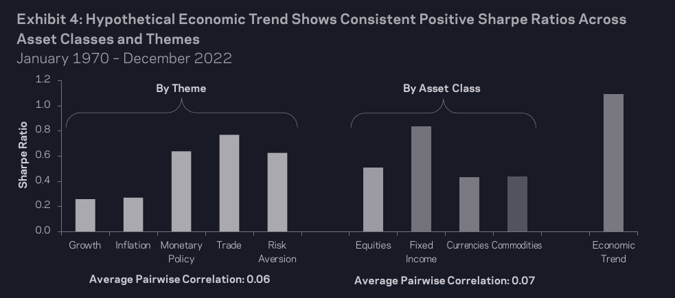
- Positive Sharpe ratio in every asset except one which was a tiny bit negative
- Economic trend had positive return during each of the 5 worst US equity drawdowns and the 5 worst US 10Y drawdowns
Economic trend and price trend
- Correlation = 0.4
- Sharpe ratios:
- economic trend: 1.1
- price trend: 1.4
- 50/50 blend: 1.5
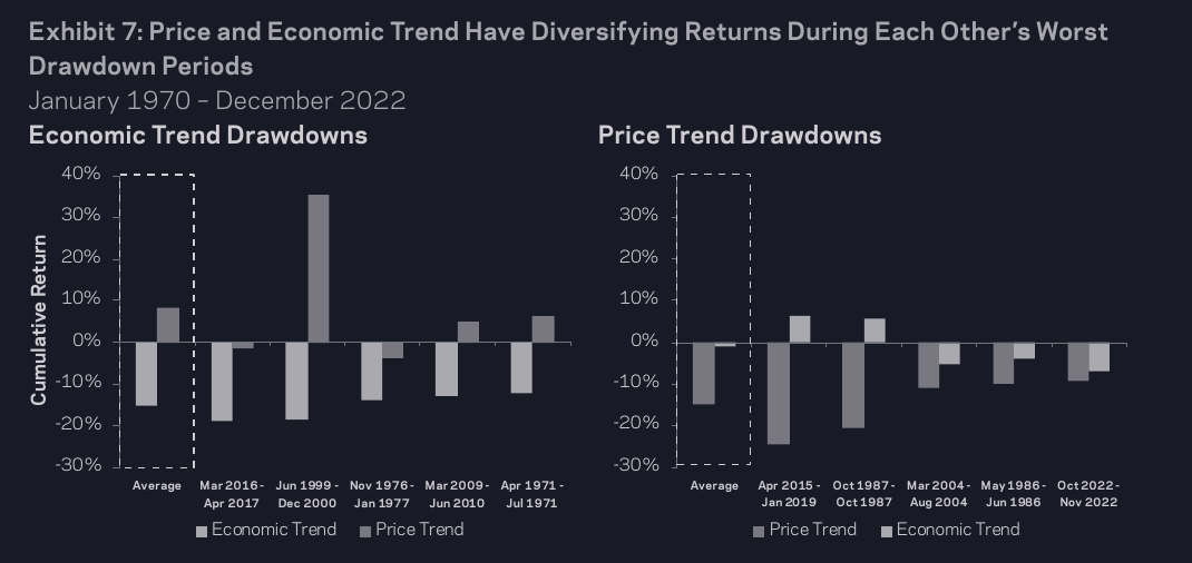
me: My thoughts
- This paper addresses some of my concerns with [2025-03-19 Wed] AQR: A Half Century of Macro Momentum (2017) by giving performance for individual signals, as well as out-of-sample performance on commodities and in the 5 years since the last paper was published
- Would still like to see a replication by an independent team. There are live funds by non-AQR firms that trade on economic trend (for example Arrow Macro Fund) but AFAIK they haven't published any research
AQR: A Half Century of Macro Momentum (2017) finance macro trend
Building a macro momentum portfolio
- Five signals based on one-year trends:
- change in GDP growth forecast
- change in inflation forecast
- FX depreciation (vs. export-weighted average)
- 2Y bond yield
- equity market return
- For each of equity indexes / currencies / govt bonds (10Y) / interest rates (3mo), go either long or short based on what the five signals indicate
- me: aren't "currencies" usually defined as local-currency 3-month rates?
- "long-short" portfolios are market-neutral and compare macro signals to the cross-sectional country average; "directional" portfolios use absolute macro signals. basically cross-sectional momentum vs. trend
- Macro momentum strategy uses half long-short, half directional
Asset class positioning based on 1-year change in momentum signals:
GDP growth inflation FX depreciation 2Y yield equity price equity indexes + - + - + currencies + + - + + govt bonds - - - - - interest rates - - - - -
Performance since 1970
| Excess Return | Stdev | Sharpe | r(US Equities) | r(US Bonds) | |
|---|---|---|---|---|---|
| 1970–2016 | 13.0% | 10.7% | 1.2 | –0.22 | 0.03 |
| 2010–2016 | 6.5% | 9.6% | 0.7 | 0.04 | 0.02 |
- Many of the data series don't start until ~1990. Performance before and after 1990 look qualitatively similar
- 0.5–0.8 Sharpe for individual asset classes; Sharpe 0.5–0.9 for individual signals
Macro momentum and traditional asset classes
- Macro momentum vs. US equities shows a "smile" much like trendfollowing
- Macro momentum performs well in drawdowns insofar as drawdowns are preceded by deteriorating fundamentals
- me: I thought equity drawdowns were a leading indicator? Could it be a leading indicator but also under-react?
- During the 10 largest increases in real yield, macro momentum returned an average of 12% annualized, compared to –14% for US 10Y Treasuries and 11% for US equities
- macro momentum returned 20% average during the top 5 increases, but had a couple negative returns during the next 5
Macro momentum and trend-following
- Both likely driven by market under-reaction to news
- They are expected to diverge at market turning points. By construction, trendfollowing will not immediately turn on a price reversal. But if price reversals are preceded by macro reversals then macro momentum may profit on average
- me: but you still can't trade at the point of a macro reversal if you're using a 1-year lookback, and in fact the 1-year price trend signal might reverse before the 1-year macro signal, because the market could react to the first (say) 3 months of macro news. although if markets under-react, you shouldn't expect a strong price reversal
- Trend-following (constructed as in "A Century of Evidence on Trend-Following Investing") and macro momentum were correlated at 0.4
- So they are indeed related, but also diversify each other
Trend-following + macro momentum had a Sharpe of 1.4, compared to 1.1–1.2 for either alone
Excess Return Stdev Sharpe Max DD Trend 12.1% 11.2% 1.1 –24% Macro Momentum 13.0% 10.7% 1.2 –22% 50/50 Combo 12.6% 9.3% 1.4 –13% - Trend-following and macro momentum each hedge each other's worst drawdowns
- me: Why? I would expect the worst times for both to occur when fundamental trends whipsaw, in which cases prices would also whipsaw
- ex: In Apr 1999–Dec 2000, macro momentum showed bad fundamentals but equities ripped anyway. When the bubble burst in 2001, trend-following suffered a drawdown, but macro momentum was correctly positioned short equities and long bonds
- me: US equity peak was in March 2000, not 2001. Maybe other asset classes peaked in 2001?
- Trend-following and macro momentum both performed well in the top 5 US equity drawdowns, with macro momentum performing slightly better in each case
Macro momentum and other alternative strategies
"Style Premia" is a market-neutral portfolio using value + momentum + carry across the same four asset classes
Excess Return Volatility Sharpe Ratio Max DD Style Premia 10.8% 11.0% 1.0 -21.3% Macro Momentum 13.0% 10.7% 1.2 -21.6% 50/50 Combo 11.9% 8.3% 1.4 -10.8% - correlation = 0.2
me: My thoughts
- These results look compelling and make me want to consider putting some money in macro momentum
- I'm not convinced yet, I would like to see:
- Does macro momentum work for each individual signal? What if you choose other signals?
- Does it work out of sample?
- What if you used other time horizons (say, 10 or 11 months instead of 12 months)?
- Some analysis of trading costs (although I expect it should be similar to price trend)
- A replication by another team—I generally trust AQR but I like to see independent replications to be safe
ReSolve: Managed Futures Carry – A Practitioner's Guide carry factors finance
Economic rationale for carry returns
- Equity: higher dividend/shareholder yield stocks should have riskier fundamentals
- Bonds: Term spreads compensate for illiquidity risk and inflation risk
- Commodities: Backwardation exists because producers hedge against price drops, and hedging provides capital for operations before the commodity is produced
- Currencies: Higher short-term rates are compensation for inflation or consumption-growth risk
Constructing carry strategies
Three ways to turn carry signals into carry strategies
- Calendar spreads: Compare front-month to back-month contracts, go long/short to harvest roll yield
- Cross-sectional carry: Buy securities with relatively high yields, short securities with relatively low yields
- Time series carry: Long positive expected carry, short negative expected carry. Portfolio may be net long or net short at various times
- For things like bonds with nearly-always positive carry, this produces positive average beta
An investor who goes long futures with high carry and hedges by shorting spot will have zero profit after all costs are considered
me: if that's true, how is carry different from just multi-asset beta?
Analytical framework
- Carry relative value is defined as the z-score of a security's carry relative to its historical carry
- We construct portfolios using either cross-sectional or time series carry, and using either raw carry or carry z-score
Performance analysis
- Basically, Time-Series Z-Score >= Time-Series Raw > Cross-Sectional Z-Score > Cross-Sectional Raw
- Multi-Strat, Multi-Sector performed ~as well as the best multi-sector strat
- best performing combo was Multi-Sector Time-Series (combining raw + z-score), but it only did slightly better than the full combo
- worst (by far) multi-sector strategy was Cross-Sectional Raw Carry—0.29 Sharpe, vs. 0.88 for the full combo
- and –60% max drawdown vs. –34%, even though both are scaled to 10% vol
- Carry did best in bonds and commodities. Had similar Sharpe in currencies, but with worse drawdowns. Equity carry had notably worse Sharpe
Performance (all targeting 10% vol):
| Return | Sharpe | Max DD | |
|---|---|---|---|
| XS Raw | 2.46% | 0.29 | -60% |
| XS Z-Score | 5.82% | 0.60 | -32% |
| XS Ensemble | 5.28% | 0.55 | -53% |
| TS Raw | 7.40% | 0.73 | -30% |
| TS Z-Score | 7.47% | 0.75 | -32% |
| TS Ensemble | 9.55% | 0.91 | -31% |
| 4-Strat Ensemble | 9.09% | 0.88 | -34% |
- All variants had correlations of +/- 0.2 to S&P 500 and US 10Y
me: My thoughts
- I was motivated to read this because I listened to interviews with Corey Hoffstein / Newfound people and they talked about how people have this idea that carry has bad drawdowns / high correlation to equity drawdowns, but it doesn’t have to be that way. But they never explained what they meant
- Having read the white paper, it looks like cross-sectional carry has bad drawdowns, but time series carry does not
- I am not a big fan of traditional (cross-sectional) carry. Time series carry looks potentially more compelling, but I don't want to change my allocation based on a single white paper
- RSSY (managed by Resolve/Newfound) presumably uses a carry ensemble. I don't know of any other carry products that do that (e.g. AFAIK AQR carry is purely cross-sectional, at least its index looks like it's cross-sectional based on the fat drawdowns)
- Resolve's backtest index has a Sharpe 1.05, Ulcer performance index (UPI) 1.90. AQR's carry index over the same period has Sharpe 0.61, UPI 0.45. I don't trust the absolute returns (it's a short-horizon backtest with no trading costs) but it's notable that Resolve-style carry had greatly reduced drawdowns—UPI was >4x higher, whereas Sharpe was <2x higher
- 2025-12-13: FrankieC has done his own backtests where time series carry did much better than cross-sectional carry
Live Q&A – Return Stacked Managed Futures Trend & Carry Flash Update finance funds
- Corey: proposed German fiscal stimulus on infrastructure and defense spending of up to 10–20% GDP (similar to COVID stimulus size)
- Adam Butler: Big proposed changes in tariffs but unclear what will be implemented
- Rodrigo Gordillo: biggest single-day move in German yields since 1990
- Rodriog: 99th–99.9th percentile moves in multiple markets
- Adam: Commodity futures yield incentivizes producers to produce more
- Corey: we use carry to forecast the total return of a market, not to just earn the carry, so we're not "clipping coupons"
- me: ? I don't get it
- Adam: carry is pro-cyclical in high-yield currencies but we don't see that across all asset classes
- Adam: historically we have seen carry make strong recoveries out of drawdowns
- Corey: we had 4 unusual policy announcements in 3 days and carry was on the wrong side of all of them
- US/Canada/Mexico tariffs, copper tariffs, EU deregulation, German stimulus
- Adam: if you own trend, you should 100% own carry. they diversify each other
- Corey: I have a lot of money in carry
Factor Investing: Long-Only vs. Long-Short (2014) factors
Long-Only vs Long-Short.pdf https://papers.ssrn.com/sol3/papers.cfm?abstract_id=2417221
- Long/short is superior theoretically, but long-only is better in most scenarios after accounting for benchmark restrictions, implementation costs, and factor decay
- Investors who want less beta should consider simply hedging out the market exposure of a long-only factor strategy, e.g. by shorting liquid futures rather than individual stocks
- me: I attempted to replicate this paper and it appears that the answer depends on which factors you look at. Replacing size with profitability makes long-short look better than long-only. See Replicating Factor Investing: Long-Only vs. Long-Short
Data and factor returns
- We consider the size, value, momentum, and low-vol factors
- For value and momentum we only look at the large-cap half to ensure good liquidity. For size factor we take NYSE 30th to 70th percentiles as small-caps
- Long-only factors e.g. "Value-RF" are the long leg of the factor minus the risk-free rate
- For low-vol factor, equal-weighted (?) long side at 130% and short side at 70% to achieve zero beta
Empirical results
Factor Sharpe ratios (gross)
US stocks 1963–2010
| Long-only | Long-short | Difference | |
|---|---|---|---|
| Mkt-RF | 0.27 | ||
| size | 0.31 | 0.24 | 0.07 |
| value | 0.49 | 0.32 | 0.17 |
| momentum | 0.49 | 0.39 | 0.1 |
| low-vol | 0.45 | 0.27 | 0.18 |
| composite (0 beta) | 0.71 | 0.73 | -0.02 |
| composite (1 beta) | 0.47 | 0.54 | -0.07 |
- Long-only worked better on individual factors, but long-short composite worked better due to greater diversification on the short side
- 0 beta had better Sharpe than 1 beta
- me: I replicated their results (using all-cap instead of large-cap) and found that this reverses if you either (1) go through 2024 (1963–2010 was a bad time for US equities) or (2) use cap-weighting instead of equal-weighting
Implementation costs and factor decay
- We assume 50 bps cost on the long side and 100 bps on the short side
- except for SMB where we assume that shorting large-caps is free
- For factor decay, we assume 100 bps market beta decay and 100 bps decay on both long and short side of factors
- me: I would assume more decay on the long side than the short side because it's more traded
- This subtracts a total of 200 bps from both long-only and long-short because long-only subtracts 100 for market and 100 for long side, and long/short subtracts 100 for each side
Net Sharpe ratios:
| Long-only | Long-short | Difference | |
|---|---|---|---|
| Mkt-RF | 0.20 | ||
| size | 0.18 | 0.02 | 0.16 |
| value | 0.34 | -0.04 | 0.38 |
| momentum | 0.35 | 0.13 | 0.22 |
| low-vol | 0.26 | -0.06 | 0.32 |
| composite (0 beta) | 0.39 | 0.14 | 0.25 |
| composite (1 beta) | 0.31 | 0.25 | 0.06 |
1-beta composite portfolio Sharpe ratios under more optimistic or pessimistic assumptions:
| Long-only | Long-short | Difference | |
|---|---|---|---|
| Optimistic decay | 0.37 | 0.34 | 0.03 |
| Pessimistic decay | 0.24 | 0.17 | 0.07 |
| Optimistic costs | 0.32 | 0.29 | 0.03 |
| Pessimistic costs | 0.29 | 0.22 | 0.07 |
(0-beta portfolios have even bigger Sharpe differences)
- Under Pessimistic Decay, long/short beta 1 has worse Sharpe ratio than Mkt-RF, and under Pessimistic Costs it only barely beats Mkt-RF
- Long-only beta 1 beats Mkt-RF even under pessimistic assumptions
Conclusion
- Long/short has additional risks in the form of leverage, counterparty risk, and lower liquidity
me: My thoughts
- Based on my own tests using the Ken French data, these results vary based on choice of factors. If you exclude the size factor and add in the quality factor, long/short beats long-only under the paper's assumptions
- I might write up a full blog post about this
- The paper might be too unfavorable toward long-short. For example perhaps the short side will see less factor decay because it's not as popular as long-only
- But my guess is the factor decay will be similar on both sides, e.g.[2018-07-28 Sat] Blitz: Are Exchange-Traded Funds Harvesting Factor Premiums? finds that there is as much money in negative-factor-loaded ETFs as in factor-loaded ETFs. On the other hand, the recent widening of the value premium was driven more by the short side than the long side, suggesting a (relatively) bigger short-side premium in the future
- Although I think this paper overstates its results, I still think long-only and long/short are both reasonable choices. I use AAVM rather than (say) AQR's long/short funds, mainly due to greater concentration and better tax-efficiency
AQR: A Changing Stock-Bond Correlation (2023) bonds finance
A Changing Stock-Bond CorrelationJPM.pdf https://www.aqr.com/Insights/Research/Journal-Article/A-Changing-Stock-Bond-Correlation
- Stocks and bonds have moved oppositely in response to growth news, and the same in response to inflation news. Stock-bond correlation depends on inflation and on the covariance of growth and inflation
- This model explains 70% of long-term variation in the US stock-bond correlation, with similar results internationally. The model is worse at explaining short-term fluctuations
- The variance in stock-bond correlation is explained by:
- 35% inflation vol
- –5% growth vol (higher growth vol = lower correlation)
- 40% growth-inflation correlation
- 29% unexplained
- current inflation level does not matter
- When Stock-Bond Diversification Fails found that trend and macro strategies perform well in both positive and negative inflation surprises
Squat University: Elbow rehab exercises fitness
Tennis elbow
https://www.youtube.com/watch?v=4Cb6JK3-co4
pain near elbow bone, on outside when supine
- Lying down, wrap band around elbow and pull tight. Squeeze fist and release 20x
- Lacrosse ball massage
- Pronated wrist curls (very light weight)
- Straight-elbow reverse crossovers (cable or light band)
- retract scapula; keep arms parallel with ground
- Standard grip exercises
Golfer's elbow
https://www.youtube.com/watch?v=9Ajfmx7qXvE
pain on crease side of elbow, toward body when supine
- Lacrosse ball massage
- if you find a spot that hurts, hold there and rotate wrist / flex grip
- Supinated wrist curls (very light weight)
- Hold band in supinated grip with forearms horizontal; stretch outward and hold 5 sec. do 10 reps
- should feel in back of shoulder. if feel in front, move elbows forward
- Same as #3 but with elbows up and forearms vertical
Swedroe: Short Sellers Are Informed Investors finance
https://alphaarchitect.com/2022/07/short-sellers-are-informed-investors/
- Shorting stocks with high short lending costs outperforms, even after accounting for short lending costs
- But unclear if the premium survives other costs like collateral and trading fees (short lending changes a lot so there's high turnover)
- AQR, Avantis, Bridgeway, Dimensional often avoid buying stocks with high short lending fees
- Dimensional excludes stocks with high fees but does not actively trade based on fees, to reduce turnover
- Avantis tries to avoid securities that have characteristics associated with high borrowing fees
The Speed of Trend-Following (2018) finance trend
Trend-following strategies
- More reactive (shorter-term) trend signals better capture short-term trends, but are more prone to whipsawing
Correlation between trend-followers
- We looked at the correlations between moving average crossover signals of different speeds, from 10 over 30 to 40 over 120
- Actual correlations are lower than the correlations you'd see if returns were IID
Actual correlations:
10x30 20x60 30x90 40x120 40x120 0.49 0.79 0.95 1 - me: the article didn't look at longer-term signals so it's kinda useless
Steve Magness: Longevity and VO2max? Does It Actually Matter? fitness
https://thegrowtheq.com/longevity-and-vo2max-does-it-matter/
- Yes VO2max is strongly associated with longevity
- But VO2max is only one component of performance and aerobic fitness
- In a meta-analysis on mortality and fitness, most studies used a performance test as a proxy for VO2max, not actual VO2max
- Harber, M. P., Kaminsky, L. A., Arena, R., Blair, S. N., Franklin, B. A., Myers, J., & Ross, R. (2017). Impact of Cardiorespiratory Fitness on All-Cause and Disease-Specific Mortality: Advances Since 2009.
- You don't need to go to a lab to test VO2max. Just improve your performance
- Measurable health improvements max out at the equivalent of a 20 minute 5K run
- This is good news. Most people can only improve VO2max ~20%, but fitness can be improved much more
- What this means about how to train:
- Train as many days a week as you can at conversational intensity
- Add one day a week of moderately hard cardio
- Once you're good at that, add a day of HARD cardio, or alternate the moderate-hard and hard workouts
- Goal isn't exhaustion, goal is to accumulate time at a hard stimulus
- Strength train twice a week
Cambria/Chesapeake managed futures seminar finance funds trend
- Jerry: only difference MFUT vs TFPN is TFPN has 50% equities, MFUT has ~25%
- MFUT is more traditional managed futures diversifier, TFPN is for crazies who want pure trendfollowing
- me: as in, you could put your whole portfolio in TFPN
- Meb: if you're not sure which fund to buy, I just say buy both. why not buy multiple managed futures ETFs?
Henselmans: Myths about posture fitness
https://www.youtube.com/watch?v=n7h8H4nGeMw
- Meta-analyses have not found a link between "bad" posture and injuries
- Saying in the same position for too long is bad for you, regardless of whether it's "good" or "bad" posture
- Anterior pelvic tilt is fine
- Posture is not caused by muscle imbalances. Muscle strength doesn't matter when your muscles are relaxed
Dynomight: air quality health
- Opening a window while cooking reduces particle levels (PM 2.5) to 1/3; a range hood reduces particles to 1/7
- Using an ultrasonic humidifier with tap water for one night is potentially as bad as smoking 5 cigarettes. Distilled water is better, but a humidifier can still get dirty and needs to be impractically clean to not spike PM 2.5
Impact of Healthy Lifestyle Factors on Life Expectancies in the US Population (2018) health fitness
https://pubmed.ncbi.nlm.nih.gov/29712712/
Gained life expectancy for males at age 50 for various activities, relative to worst category
0.1–1 hrs/week exercise 3 >6 hrs/week exercise 7 not smoking 10 2nd quintile diet quality 1 4th quintile diet quality 2 5th quintile diet quality 4 - BMI 18.5–23 has same life expectancy as 23–25. 25–30 is <1 year worse, 30–35 is 3 years worse, >35 is 5 years worse
- Being low-risk on five factors (exercise, smoking, diet, alcohol, BMI) had +13 years life expectancy vs. being high-risk on all factors
- Data obtained from questionnaires, except for BMI which was measured. Based on skimming methodology, I think they didn't control for any confounders
Jeff Nippard: The best and worst shoulder exercises fitness
https://www.youtube.com/watch?v=SgyUoY0IZ7A
(for building big delts)
- best for side delts: cable lateral raise
- best for rear delts: reverse cable crossover
- best for front delts: machine shoulder press
Stronger By Science: Meta-analyses are the gold standard for evidence, but what's the value of gold these days? science rationality
https://www.strongerbyscience.com/meta-analyses/ Kadlec, D., Sainani, K. L., & Nimphius, S. (2022). With Great Power Comes Great Responsibility: Common Errors in Meta-Analyses and Meta-Regressions in Strength & Conditioning Research.
Kadlec et al. (2022)
- The study reviewed the 20 most-cited meta-analyses in strength and conditioning. 85% of them contained at least one statistical error
- An analysis that does these can still be useful, but be aware of the limitations
Ignoring outlier studies: 25%
- One or a few studies might have outrageous results that skew the average
- These will show up on a funnel plot
Using standard errors instead of standard deviations: 45%
- ex: Effect size is calculated by dividing by the standard deviation, not standard error
- If the forest plot has studies with weirdly large effect sizes, that suggests the researchers used stderr instead of stdev
Ignoring within-study correlation (failing to account for correlated observations): 45%
- Meta-analyses often treat two groups within the same study as independent, which is double-counting
Focusing on within-group rather than between-group results: 45%
- i.e. comparing intervention group before and after intervention, rather than intervention group minus control group, before and after intervention
Failing to account for within-study variance (failing to weight studies): 40%
- Standard approach is inverse variance weighting, which functionally means studies are weighted by sample size
The meta-analysis checklist
Are the data reported at the group level or participant level?
- Participant-level analyses are better, but they're usually not possible
Are there enough studies or participants to draw strong conclusions?
- Does >50% of the weight come from a single study?
- If the studies are homogeneous, that's good because the meta-analysis can get a more reliable effect, but it's bad because you can't tell if the results will generalize
Are these studies similar enough to even think about combining their data?
- If the studies used very different methods and you combine them, what exactly are you looking at?
Are the measured outcomes similar enough to even think about combining them?
- ex: Can we really treat isometric grip strength as comparable to 10RM squat? Answer depends on context
Have effect sizes been calculated correctly?
- Effect sizes in different studies are usually not measuring the same thing. A meta-analysis has to standardize them, e.g., by converting to Cohen's d
- Some meta-analyses calculate within-group effect size when it would be more appropriate to calculate between-group effect size
- Should divide by stdev of baseline, not stdev of change. Ex: group can bench 100 +/- 20 kg at baseline, and a supplement increases their bench by 3 +/- 5 kg. The effect size could be presented as 3/5 or as 3/20
- me: I think the correct answer is 3/20 if you look at the change in means, and 3/5 if you look at the paired changes for each individual person. but not sure
Have they used an appropriate statistical model?
- Did they make the appropriate decision to use a fixed-effect or random-effects model?
- Usually, random-effects is better
- Fixed-effect means there is one true effect size. Random-effects means there are multiple true effect sizes for different sub-populations and the meta-analysis wants to find the population average
- Did the researchers appropriately account for confounding variables?
Are there any implausibly large effects, implausibly narrow CIs, or outliers?
- Look at the forest plot and funnel plot
Is there a lot of unexplained heterogeneity?
- If a study looks very different from the average, is that just because it's small? Or is there some difference that could influence the result?
- If you can't identify any reason for the difference, that's an issue for our estimate of the average effect
Milo Wolf training volume meta-analysis fitness
https://www.youtube.com/watch?v=6zQilDS-NBA
(the paper isn't out yet)
- Doubling number of sets increases hypertrophy by 50%. Holds between 5 and 30 sets per week
- Fractional sets model, where e.g. a set of rows counts as half a set of biceps, had better predictive power than counting rows as 1 set or 0 sets
examine.com: Is saturated fat bad for your health? health
https://examine.com/faq/is-saturated-fat-bad-for-your-health/
- WHO (2016) meta-analysis: replacing carbs/MUFA/PUFA with SFA had mostly-consistent bad effects on biomarkers (exception: carbs -> SFA lowered triglycerides; anything -> SFA raised HDL but by less than LDL)
- Consistent effects across a wide range of blood-lipid values and saturated-fat intakes (1.6–24.4% of calories) and across studies
- LDL-C (total volume of cholesterol inside LDL particles) isn't as predictive as LDL-P (total number of LDL particles). The more particles, the more likely it is that some will get stuck in arteries
- LDL-P is estimated by apoB because there is one apoB particle per LDL particle
- There is a mechanism where LDL could increase inflammation, but systematic review failed to find an effect on a variety of inflammatory biomarkers
- Meta-analyses of observational studies have failed to find SFA <> heart disease association
- One RCT meta-analysis found SFA caused heart disease, but another only found a link when replacing SFA with omega-3s + omega-6s, not omega-6s alone
- Replacing SFA with whole grains or plant-based MUFAs is associated with reduced heart disease risk, but replacing with refined grains or animal-based MUFAs is not
DIAAS table health
Limiting amino acids for various proteins (for age 6mo–3y)
Comprehensive overview of the quality of plant- And animal-sourced proteins based on the digestible indispensable amino acid score, Table 2 (see also full article)
- limited by lysine: wheat, corn, rice, hemp, oat
- limited by methionine + cysteine: fava bean, pea, soy
- limited by leucine: quinoa[1]
- Note: Figure 2 says DIAAS scores for adults are higher across the board than for 6mo–3y (e.g. soy is >100 instead of 91)
- FAO report Table 5 gives recommended mg/g by age group. It recommends much less leucine/lysine/methionine for adults than for 6mo-3y, so the limitations from the above paper systematically underestimate protein quality
[1] Quinoa protein: Composition, structure and functional properties
DIAAS child
note: hemp protein tryptophan value is unknown, so I just put it as 100
| Protein source | Histidine | Isoleucine | Leucine | Lysine | Met + Cys | Phe + Tyr | Threonine | Tryptophan | Valine | DIAAS | Limiting AA |
|---|---|---|---|---|---|---|---|---|---|---|---|
| Soy | 119 | 124 | 102 | 96 | 91 | 147 | 105 | 132 | 95 | 91 | Met + Cys |
| Wheat | 118 | 91 | 87 | 48 | 127 | 109 | 78 | 127 | 92 | 48 | Lys |
| Pea | 99 | 101 | 87 | 110 | 70 | 116 | 94 | 77 | 83 | 70 | Met + Cys |
| Fava bean | 108 | 106 | 95 | 95 | 55 | 119 | 91 | 68 | 83 | 55 | Met + Cys |
| Hemp | 124 | 106 | 85 | 54 | 121 | 131 | 87 | 100 | 99 | 54 | Lys |
| Corn | 110 | 90 | 162 | 36 | 126 | 140 | 86 | 52 | 90 | 36 | Lys |
| Rice | 93 | 89 | 80 | 47 | 104 | 119 | 75 | 114 | 95 | 47 | Lys |
| Potato | 100 | 156 | 143 | 122 | 115 | 210 | 165 | 128 | 138 | 100 | NA |
| Oat | 91 | 100 | 94 | 57 | 151 | 135 | 85 | 110 | 102 | 57 | Lys |
| Rapeseed | 107 | 90 | 78 | 67 | 125 | 92 | 97 | 106 | 92 | 67 | Lys |
| Lupin | 121 | 104 | 89 | 75 | 68 | 121 | 97 | 72 | 78 | 68 | Met + Cys |
| Canola | 105 | 93 | 79 | 72 | 121 | 97 | 97 | 112 | 87 | 72 | Lys |
| Gelatin | 34 | 34 | 35 | 60 | 27 | 36 | 46 | 2 | 46 | 2 | Trp |
| Whey | 85 | 166 | 138 | 131 | 132 | 101 | 174 | 180 | 116 | 85 | His |
| Egg | 101 | 129 | 103 | 133 | 123 | 144 | 106 | 129 | 105 | 101 | NA |
| Casein | 147 | 153 | 141 | 134 | 117 | 201 | 130 | 159 | 148 | 117 | NA |
| Pork | 197 | 153 | 122 | 157 | 128 | 148 | 145 | 144 | 117 | 117 | NA |
reference values (mg per g of protein)
| Age group | Histidine | Isoleucine | Leucine | Lysine | Met + Cys | Phe + Tyr | Threonine | Tryptophan | Valine |
|---|---|---|---|---|---|---|---|---|---|
| 0.5–3y | 20 | 32 | 66 | 57 | 27 | 52 | 31 | 8.5 | 43 |
| >3y | 16 | 30 | 61 | 48 | 23 | 41 | 25 | 6.6 | 40 |
DIAAS adult
| Protein source | Histidine | Isoleucine | Leucine | Lysine | Met + Cys | Phe + Tyr | Threonine | Tryptophan | Valine | DIAAS |
|---|---|---|---|---|---|---|---|---|---|---|
| Soy | 149 | 132 | 110 | 114 | 107 | 186 | 130 | 170 | 102 | 102 |
| Wheat | 148 | 97 | 94 | 57 | 149 | 138 | 97 | 164 | 99 | 57 |
| Pea | 124 | 108 | 94 | 131 | 82 | 147 | 117 | 99 | 89 | 82 |
| Fava bean | 135 | 113 | 103 | 113 | 65 | 151 | 113 | 88 | 89 | 65 |
| Hemp | 155 | 113 | 92 | 64 | 142 | 166 | 108 | 129 | 106 | 64 |
| Corn | 138 | 96 | 175 | 43 | 148 | 178 | 107 | 67 | 97 | 43 |
| Rice | 116 | 95 | 87 | 56 | 122 | 151 | 93 | 147 | 102 | 56 |
| Potato | 125 | 166 | 155 | 145 | 135 | 266 | 205 | 165 | 148 | 125 |
| Oat | 114 | 107 | 102 | 68 | 177 | 171 | 105 | 142 | 110 | 68 |
| Rapeseed | 134 | 96 | 84 | 80 | 147 | 117 | 120 | 137 | 99 | 80 |
| Lupin | 151 | 111 | 96 | 89 | 80 | 153 | 120 | 93 | 84 | 80 |
| Canola | 131 | 99 | 85 | 86 | 142 | 123 | 120 | 144 | 94 | 85 |
| Gelatin | 42 | 36 | 38 | 71 | 32 | 46 | 57 | 3 | 49 | 3 |
| Whey | 106 | 177 | 149 | 156 | 155 | 128 | 216 | 232 | 125 | 106 |
| Egg | 126 | 138 | 111 | 158 | 144 | 183 | 131 | 166 | 113 | 111 |
| Casein | 184 | 163 | 153 | 159 | 137 | 255 | 161 | 205 | 159 | 137 |
| Pork | 246 | 163 | 132 | 186 | 150 | 188 | 180 | 185 | 126 | 126 |
| Protein source | DIAAS |
|---|---|
| Soy | 102 |
| Wheat | 57 |
| Pea | 82 |
| Fava bean | 65 |
| Hemp | 64 |
| Corn | 43 |
| Rice | 56 |
| Potato | 125 |
| Oat | 68 |
| Rapeseed | 80 |
| Lupin | 80 |
| Canola | 85 |
| Gelatin | 3 |
| Whey | 106 |
| Egg | 111 |
| Casein | 137 |
| Pork | 126 |
| Wheat/Pea 70/30 | 79 |
| Pea/Fava/Hemp | 88 |
How to fix wheat protein
Take one 500mg lysine pill per 28g wheat protein to push the DIAAS up to 94. (= 0.5 / (48 / 1000 * (0.94 - 0.57)))
UW/NIA collab: Caloric restriction improves health and survival of rhesus monkeys (2017) health
- University of Wisconsin (UW) longitudinal study found that calorie restriction (CR) increased survival of rhesus monkeys
- National Institute of Aging (NIA) study found no significant effect
- This paper describes differences in the study designs. Taken together these results confirm the health benefits of CR
- me: I don't see how this conclusion is justified
Methodology
- UW study gave each money food at libitum, then in the CR group restricted calories proportionally for each individual based on their intake
- NIA study gave control group a fixed amount of food based on National Research Council guidelines, and gave CR group 30% less food than that
- calorie intake was determined by weighing uneaten food, as reported in a different paper on the same study (Age-related decline in caloric intake and motivation for food in rhesus monkeys, 2005)
- the fixed upper intakes likely prevented the worst right-tail outcomes
Results
- UW ate processed foods, NIA ate whole foods. UW ate primarily whey protein, corn, sucrose (45%), corn oil, cellulose (5g). NIA ate soybean and fish meal, wheat, corn, sucrose (7%), cellulose (6-9g)
- NIA split monkeys into juvenile/adolescent (J/A) and old. CR reduced mean/median lifespan 2–3 years in J/A group but had a small and mixed effect in old group (Figure 1 & Table 3)
- me: possibly b/c CR increases premature deaths and decreases late deaths. should look at causes of death (accidental/infectious vs. chronic disease)
- UW control (ad libitum) had highest bodyweight; UW CR and NIA control + CR had similar bodyweights for female, and for males NIA CR had lower bodyweights than NIA control (Figure 2). Body fat % had similar relationship to bodyweight (Figure 3)
- even though NIA CR group ate ~25% fewer calories than NIA control group (Figure 4)
- me: weird that NIA females had only small difference in bodyweight, but NIA males had large difference
- me: for NIA the number of individuals at each age appears to fluctuate randomly. how is that possible?
- Both UW and NIA showed later onset of all-cause age-related morbidities in the CR group, but with the difference being greater for UW (Figure 6). Cancer and diabetes followed the same pattern, but for NIA, CR had more heart disease than control
- both NIA groups had less heart disease than either UW group. UW and NIA CR groups had equal cancer rates
- me: Monkeys eat less as they age. Therefore, the caloric upper bound in the NIA control group should be less restrictive for monkeys whose bound is set when they're young, and therefore CR should show a more prominent effect in NIA older monkeys. That's kind of the opposite of what we see: in J/A cohort, CR is harmful, but in old cohort, there's no consistent effect
- me: some concerns about extrapolating these results
- lab conditions are different from real world in many ways
- the monkeys were sedentary. they were individually housed in small cages (NIA 2005). it seems likely that physical activity largely negates the benefits of calorie restriction (e.g. hunter-gatherers who eat a lot of sugar but are physically active have very low rates of diabetes: Hunter-gatherers as models in public health)
- physical activity was tested in a different paper, but it was tested inside a metabolic chamber that was about the same sizes as the cages, i.e., too small for meaningful exercise (Long-term calorie restriction decreases metabolic cost of movement and prevents decrease of physical activity during aging in rhesus monkeys, 2013)
NIA study
Impact of caloric restriction on health and survival in rhesus monkeys: the NIA study
- In the old-onset cohort, CR group did not have better survival, but did have lower triglyceride, cholesterol, and glucose levels
- In the young-onset (J/A) cohort, CR group did not have better survival or better biomarkers, but did (maybe) have less age-related disease (p=0.06) (age-related disease was not reported for old-onset cohort, for some reason)
me: My thoughts
See the relevant section of Outlive: A Critical Review
Dialogue on Donation Splitting (2023) causepri
https://forum.effectivealtruism.org/posts/x2iT45T5ci3ea9yKW/dialogue-on-donation-splitting between JP Addison and Eric Neyman
JP
- Standard argument against splitting: for small donors, marginal cost-effectiveness is unlikely to change between first and last dollar. This seems right to me
Eric
- I believe you should donate to charities in proportion such that, if all like-minded EAs donated in that proportion, the outcome would be best
- If everyone lump-donates based on the funding situation as of several months ago, then the top charity receives all the money. If everyone proportionally donates, then every charity receives the correct amount of money
JP
- I like this position. Some conceivable objections:
- EAs' conclusions about where to donate might not be that correlated
- Are we setting a norm for all EA, or just for the individual who asked my opinion? I want to avoid unilaterally doing something that only pays off when everyone does it, unless everyone is going to do it
Eric
- I agree that those are cruxes
JP
- wrt correlation, what type of correlation are we interested in? All EAs? Donors to a particular cause? etc.
- Could ask GiveWell, GWWC, etc. about the correlation among donations they have visibility into
Eric
- The relevant question is, is the correlation strong enough to collectively hit diminishing returns?
- Correlation within a cause area is a bigger deal
JP
- Agree that within-cause correlation is the natural unit of analysis. Cross-cause I don't think donation splitting makes sense
Eric
- Could get correlations from the EA Forum donation election
- This conversation has moved me from correlation being a medium-large problem to a small-medium problem. Still confused about how to think about correlation
JP
- In terms of decision theory, I lean toward lump sum because humans tend to reason in various messy ways, so your own reasoning isn't much evidence about other people's reasoning
Eric
- Insofar as we're making a public recommendation, we should tell people to coordinate on some sort of mild donation splitting strategy
Menno Henselmans: Elbow pain when training triceps fitness
https://www.youtube.com/watch?v=zlGEliRQBsc
- Do high-rep sets (>12 reps). They stimulate tendons much less
- I like sets of 30
- Go hard or go home
- As in, if you can't do sets of 30 at close to failure, just don't train triceps. You will still hurt yourself and also not get muscle stimulation
- Use slow tempo
- Forces muscles to act as brakes instead of tendons
- Can help to avoid complete lockout
- Keep forearms vertical / use wide grip
- Try changing your grip or wrist rotation
looking into the Momma et al. studies on resistance training decreasing all-cause mortality health fitness
https://todayspractitioner.com/wp-content/uploads/2022/09/Muscle-Strengthening-Study-PDF.pdf
- See also [2023-07-06 Thu] Nuckols: What is the optimal dose of resistance training for longevity?
- Dose-Response relationship was evaluated using (in order of weight) Patel, Grontved, Kamada, Stamatakis, Liu, Porter
- Momma et al. assessed the quality of evidence on resistance training and all-cause mortality, as well as most mortality subcategories, as "very low". The only exception was the evidence on diabetes, which they assessed as "low"
- Porter found mortality benefits to some activities like running and aerobics, but no benefits to other activities like weight training but also bicycling, gymnastics, swimming, and basketball. which is pretty suspect
- Patel found similar HR for 0-1h and 1-2h of resistance training (0.88 and 0.90), with worse HR (1.01) for >2h, when controlling for BMI, aerobic activity, and other stuff
- >2h had good hazard ratio when not controlling for all that stuff, but the controlled model is more relevant than the uncontrolled model
- participants were older (aged 50–74 at start of study). 74,462 eligible participants, but only 3470 reported >2h resistance training
- comorbidity score (high blood pressure + type 2 diabetes + high cholesterol) monotonically decreased with resistance training groups: average scores 1.218, 1.100, 1.095, 1.086. calculated from the bottom of Table 2. the uncontrolled numbers for all-cause mortality show all HR < 1, but >2h group is worse than 0–1h or 1–2h so the comorbidity score is more optimistic for high resistance training, although surely much of this is explained by confounders like higher aerobic activity (which was also monotonic)
- Grontved found monotonic relationship with resistance training and diabetes in women but AFAICT it did not look at all-cause mortality
- note: this study is the wrong Grontved but still
- Grontved found monotonic relationship with diabetes in men in all four models (progressively adjusting for more confounders)
- weirdly, weight training monotonically decreased diabetes association for under age 65 (p=0.002), but monotonically increased for >65 (p=0.6) (except that for >65, resistance training still had lower diabetes risk than no resistance training even for >150 min/week group). eyeballing CIs, looks like weight training volume is just barely significantly worse for >65 than for <65 (right around p=0.05). this suggests that age at least partially explains the higher mortality for high resistance training
- meta note: most of these papers used the same cohort studies as cited in Eat, Drink, and Be Healthy (Nurses' Health Study, Health Professionals Follow-Up Study, Cancer Prevention Study II)
The physical activity paradox: six reasons why occupational physical activity (OPA) does not confer the cardiovascular health benefits that leisure time physical activity does health fitness
https://bjsm.bmj.com/content/52/3/149
Six hypotheses for why leisure time physical activity (LTPA) improves health, but OPA does not:
- OPA is of too low intensity or too long duration
- Improving fitness requires moderate intensity (>60% max heart rate)
- OPA elevates 24-hour heart rate
- Acute elevated heart rate is good, but long-term elevated heart rate is bad
- OPA including heavy lifting or static postures elevates 24-hour blood pressure
- OPA is often performed without sufficient recovery time
- OPA is often performed with low worker control
- Poor health may be due to heat stress, dehydration, etc.
- OPA increases inflammation
me: some of these are causally intertwined: OPA would increase heart rate/blood pressure/inflammation because it is too long duration/has insufficient recovery time
Austin Baraki finds hypothesis #5 the most plausible
Volume for Muscle Hypertrophy and Health Outcomes: The Most Effective Variable in Resistance Training health fitness
(My key question: does resistance training reduce mortality at sufficiently high volumes?)
- RCT: 3 sets of 8 exercises per week had better health outcomes than 1 set of 8 exercises
- me: 24 sets still isn't that much volume. standard bodybuilding recommendation is 10–20 sets per muscle group, not total
- Dose-response relationship for type 2 diabetes for every 60 min per week (but we already knew that)
- High volume reduced sarcopenia in the elderly up to 39 sets per week
- me: This paper only cited 3 outcomes. It's decent evidence but not conclusive
Iñigo San-Millán & Petter Attia: Deep dive back into Zone 2 Training fitness
- Zone 2 is when you stress mitochondria and oxidative capacity the most. You recruit mainly slow-twitch muscle fibers, burn the most fat, and stimulate the most oxidative phosphorylation (so you're using both fat and glucose)
- If someone breathes into a VO2 meter, the ratio of VO2/VCO2 tells you how much energy is coming from fat oxidation vs. glycolysis. When burning fat, you still consume oxygen but you emit less CO2
- Elite athletes can burn more fat because their mitochondria are more efficient at converting fat to ATP
- Glycolysis produces lactate
- Lactate causes cancer to grow faster; exercise improves the body's ability to clear lactate
Mike Israetel: What I've changed my mind about (Thomas DeLauer podcast) health fitness
https://www.youtube.com/watch?v=sLxo8mDW2QY
- I used to believe fasting had longevity benefits. I still sort of believe that, but the benefits almost entirely come from caloric restriction, not fasting per se
- Having excess nutrients floating around in your bloodstream is bad for longevity (it increases inflammation). Fasting fixes this but so does a calorie deficit, and exercise (esp. steady-state cardio) works even better
- I used to believe it was good to eat as many meals per day as possible. Now I believe there are only slight benefits to eating more than 3 meals, and basically no benefit to eating more than 4 meals (unless you want to)
- The food stays in your digestive system for a while so there's no point in eating more than 3–4 meals
- Unless you have protein powder, which fully digests after ~2 hours. Protein alone digests faster than protein with carbs/fat
- I used to think you needed full ROM, now I think the stretched position is best for hypertrophy and full ROM on the contracted side isn't as important
- Sometimes lockout is a rest so it's better to not lock out when controlling for # reps
- I used to care a lot about glycemic index. But when you eat a meal with a mix of macros, high-GI foods behave like they have low GI. White rice only spikes your blood sugar if you eat it by itself
- I used to try to apply maximum recoverable volume for advanced lifters to novices. Novices can recover from more
- The limiting factor is usually systemic fatigue, not per-muscle fatigue. Recent studies show you can train 30–50 sets per week if you only train one muscle group
PG: The Best Essay
https://paulgraham.com/best.html
- Start from a question
- It probably won't work to choose an important-sounding topic and random because you need an edge, a new way in
- Start from something that puzzles you, even if it's minor
- Start writing anything about it. Writing converts your ideas from vague to bad. Once you see the badness, you can fix it
- Writing is linear, so you have to pick which branch to follow. Pick whichever branch seems most novel and most general, and keep writing. Be willing to backtrack and delete a lot of text
- Most questions can produce good essays, but only some produce great ones. Can we predict which questions will yield great essays? Considering how long I've been writing essays, it's alarming how novel that question feels
- One thing I like in an initial question is outrageousness (e.g., counterintuitive or overambitious or heterodox)
- I don't systematically generate lists of questions; I write about whatever I'm thinking about. But if the initial question matters, I should care about it
- Go a step earlier: write about whatever pops into your head, but try to ensure that what pops into your head is good
- For you to have insight into a topic, it needs to be something you've thought about anyway
- Get a breadth of ideas by reading, and talking to people who help you have ideas; get depth by doing (by solving problems)
- Good questions require inspiration, but good answers can be got by sheer persistence: keep rewriting until you get them
- Unfortunately, the questions are the harder thing to get
Humans are not automatically strategic self_optimization rationality
https://www.lesswrong.com/posts/PBRWb2Em5SNeWYwwB/humans-are-not-automatically-strategic
- Why will a randomly chosen eight-year-old fail a calculus test? Because most possible answers are wrong, and there is no force to guide them to the correct answers
- Why do most of us pursue our goals through ineffective routes? Because most routes are ineffective, and there is no strong force pushing us toward effective routes
- Useful things to do if you have goals:
- Ask yourself what you're trying to achieve
- Ask yourself how you could tell if you achieved it
- Be curious about information that would help you achieve your goal
- Gather that information (e.g., by asking how other people have achieved similar goals, or by tallying which strategies have and haven't worked)
- Test many conjectures for how to achieve the goals, including methods that aren't habitual for you
- When not exploring, focus on which methods work best
- Use short-term cues to bolster motivation so you don't get stopped by intermittent frustrations
Fundamentally, Momentum Is Fundamental Momentum momentum
https://www.nber.org/system/files/working_papers/w20984/w20984.pdf
(incomplete notes)
- SUE = long/short portfolio formed on (quarterly) earnings surprises
- SUE has positive alpha on top of UMD but UMD has negative alpha on top of SUE
Conditional strategies
- UMD controlling for SUE has worse return than UMD (but still positive). SUE controlling for UMD has better return than SUE
AlphaArchitect: Multi-factor strategies: portfolio blending vs. signal blending / separate or combined? (compilation) factors
compilation of 1, 2, 3, 3b (AQR), 3c (Newfound), 4, 5, 6
- [1] We found that separate beat combined for a top decile EBIT/EV + momentum strategy in mid to large caps 1963 to 2013 (Sharpe 0.66 vs. 0.72)
- [2] A paper found that portfolio blending works better with low (<90%) exposure or low (<8%) active risk, and signal blending works better with high factor exposure or high active risk
- Tested using various combinations of factors
- AQR: For long-only investing, signal blending has a higher information ratio than portfolio blending at any given level of tracking error
- Newfound: Value and momentum operate over different time horizons. If we blend signals, we run the risk that the high-turnover factor dominates the selection process
- Half-life of a momentum signal was 0.27 years; for value signal was 3.76 years
- me: I don't see why this matters
- [3] For long/short factor portfolios 2001 to 2017, we found that signal blending beat portfolio blending
- [4] We formed separate portfolios by taking the top 50 to 200 value or momentum stocks and a combined portfolio by taking the top 100 to 400 stocks by a combined value+momentum ranking. We used E/P instead of EBIT/EV and did not exclude utilities/financials. All equal-weighted; 1992 to 2021. For US equities, separate had 3pp higher CAGR than combined with 100 stocks, and 1pp higher CAGR with 400 stocks. International equities had a similar result but with only a 1.5pp difference. Sharpe ratios were similar for separate vs. combined and not consistently better for one or the other
- [5] Bender & Wang found that signal blending beat portfolio blending (on CAGR and Sharpe) for long-only cap-weighted portfolios
- The difference compared to AA's studies ([1], [3]) may be because the effect reverses in sufficiently concentrated portfolios, or because AA use EBIT/EV instead of B/M
- me: perhaps portfolio blending being better requires equal-weighting
- [6] Reschenhofer didn't look at portfolio blending but he did find that signal blending portfolio behavior is sensitive to construction/rebalancing rules, which could explain some of the differences seen in previous studies
My summary
- Most studies found that combined works better than separate
- AA found that separate works better than combined for their specific implementation style. Reason for the difference is unclear. Some possibilities: equal weighing; long only; different metric (EBIT/EV instead of B/M)
- Difference is small either way. That plus the inconsistent results suggests it doesn't really matter
AQR: The Role of Shorting, Firm Size, and Time on Market Anomalies factors
Role of Shorting, Firm Size, and Time on Market Anomalies.pdf
(skimming)
- Long positions comprise 60% of value and momentum profits
- me: abstract says 60% of value and half of momentum, but Table 5 says it's 60%/60% for global stocks (and somewhat different numbers in different regions)
- Shorting becomes less important for momentum and more important for value as firm size decreases
- The value premium decreases with firm size and is weak among mega-caps; momentum has no reliable relationship with size
- These results hold over 80 years of US equity data and 40 years international equity data
Introduction
- Value premium is insignificant in the 40% largest stocks
Interaction of firm size with value and momentum
| Small 20% | Large 20% | |
|---|---|---|
| value alpha | 12.99% (4.52) | 2.19% (1.14) |
| value % long side | 47.4% | 89.9% |
| momentum alpha | 13.12% (5.59) | 10.24% (4.23) |
| momentum % long side | 70.9% | 38.3% |
three big studies on BMI health
(I found the first one from searching, and latter two were cited by Eat Drink & Be Healthy)
Association of BMI with overall and cause-specific mortality: a population-based cohort study of 3-6 million adults in the UK (2018)
https://www.thelancet.com/journals/landia/article/PIIS2213-8587(18)30288-2/fulltext
- me: Authors are aware of the confounding issues with illnesses causing weight loss so I assume they accounted for it but I didn't read in detail
- For most specific causes, BMI has a U-shaped mortality, with the right side being worse than the left side
- Causes where the left side is worse: lung cancer, prostate cancer, neurological (dementia etc.), falls, suicide, interpersonal violence
- Causes with a symmetric U shape: musculoskeletal, accidents (aggregate, including falls), respiratory
- Pretty much everything else is higher on the right: all cancers, blood/endocrine, cardiovascular
- Confirms that the healthiest BMI range is 18–25
- All-cause mortality is minimized at 23 kg/m2 under age 70, and BMI 25 over 70
- me: From graphs, looks like ideal BMI slowly increases with age from ~22 at <50 to to ~26 at >80; and is slightly lower for men than for women, and women can tolerate BMIs up to ~28 without much impact on mortality
Body-mass index and all-cause mortality: individual-participant-data meta-analysis of 239 prospective studies in four continents
https://www.thelancet.com/journals/lancet/article/PIIS0140-6736(16)30175-1/fulltext Supplementary Appendix
- Healthiest BMI is 20 to 25. Mortality significantly increases just below or above this range
- Table 3 finds mortality is minimized at 22.5–25. 20–22.5 is nearly identical, and mortality considerably increases <20 and >25
- me: look at the hazard ratios, not the deaths per participant, because deaths per participant needs to be adjusted in various ways
Hazard ratios for cause-specific mortality (appendix eTable 15)
18.5–20 20–22.5 22.5–25 25–27.5 cardiovascular disease 1.14 0.98 1.00 1.11 coronary heart disease 0.95 0.89 1.00 1.18 stroke 1.15 1.01 1.00 1.05 respiratory disease 1.73 1.22 1.00 1.00 cancer 1.01 0.96 1.00 1.05 - me: Notice the heterogeneity: 20–22.5 is better for heart disease and cancer, but much worse for respiratory disease
Ideal BMI by age (appendix eFigure 2)
Age BMI 35–49 20–22.5 50–69 22.5–25 70–89 25–27.5 - Ideal BMI by sex (appendix eFigure 3) is the same for both sexes, but females have lower hazard ratios across the board (i.e. lower penalty for being under- or over-weight)
- Across 6 steps of successively stricter inclusion criteria, low-BMI hazard ratios consistently go down and high-BMI hazard ratios consistently go up. 20–22.5 starts out with HR ~1.2 and descends to 1.01. 18.5–20 starts at HR ~1.4 and descends to ~1.2
- me: Presumably we still aren't perfectly controlling for everything. Extrapolating the trend suggests that 18.5–22.5 is healthier than the data suggest
BMI and all cause mortality: systematic review and non-linear dose-response meta-analysis of 230 cohort studies with 3.74 million deaths among 30.3 million participants (2016)
https://www.bmj.com/content/353/bmj.i2156
- Ideal BMI was 23–24 in never-smokers, 22–23 in healthy never-smokers, and 20–22 in never-smokers in studies with >20 years of follow-up
- me: I believe the argument is that low BMI could be caused by undiagnosed illnesses that don't show up in shorter-term studies. Sounds plausible but I don't fully understand why using longer studies fixes this problem. Perhaps the idea is you filter out anyone who dies within the first 5 years, which eliminates most people who had some undiagnosed disease
Dynomight: Does gratitude increase happiness? self_optimization psychology
https://dynomight.net/gratitude/
- Gratitude is correlated with happiness in observational studies, but there are other explanations (gratitude and reported life satisfaction are both determined by an innate happiness set point; both are predicted by +O+C+E+A-N; happier people have more to be grateful for)
- Gratitude journaling does increase reported happiness in studies, but so does doing literally anything. It has a small effect compared to neutral activities like listing what activities you did, and an even smaller effect compared to positive activities like imagining your ideal self
- Funnel plot suggests publication bias
- Adjusting for publication bias, one meta-analysis found it halved the effect size; another found it reduced the effect size to zero
AQR: Fact, Fiction, and the Size Effect (2018) finance factors
Fiction: The size effect is one of the strongest factors
- In our replication of the original size effect paper Bantz (1981) that looked from 1936 to 1975, regressing size against CAPM, we got an SMB t-stat of only 1.21 and negative alpha; and a top minus bottom decile t-stat of 1.78 and 2.5% alpha (t=0.66)
- Much of small-cap outperformance is just beta (or all of it, if you use SMB construction)
- Why is our result weaker than that of Bantz (1981)?
- Older databases had more errors such as delisting bias
- me: small-caps probably delist more than large caps, creating an illusion of better small-cap performance
- Older databases had more errors such as delisting bias
- 1926–2017 SMB looks about the same but alpha t-stat is still non-significant
- Other major factors (HML, MOM, RMW, BAB) all have good alpha t-stats
Fact: The size effect has disappeared or weakened since its discovery
- me: their data actually shows that it slightly strengthened but it's still weak
Fiction: The size effect is robust to how you measure size
- Measuring size by book equity, book assets, sales, PPE, or number of employees resulted in no reliable size premium
- me: most of these are gonna have negative loading on the value factor so I am not sure this approach is valid
Fact: The size effect is dominated by a January effect
- If you ignore January, SMB has 0.0% return 1927–2017
Fiction: The size effect works in other equity markets
- SMB is negative in Europe, global, and North America; marginally positive in Pacific; and somewhat but non-significantly positive in global ex-US
- me: I don't get how it's negative in global but positive in global ex-US
- SMB is negative in 13/23 individual countries
- SMB is larger than in US in emerging markets (data starts in 1994) (alpha t-stat 1.27)
Fact: The size effect is either not applicable or does not work for other asset classes
- Country equity index SMB (long small countries, short big countries) has a modest size premium (alpha t-stat 1.68)
- Corporate bond SMB has negative alpha
- Currency SMB (using GDP to measure size) has a weak premium in developed markets (alpha t-stat 0.41) and a weak negative premium in emerging markets (alpha t-stat –0.95)
Fact: The size effect mostly comes from microcap stocks
- Removing stocks with size < $5M eliminates the small-cap premium
- Decile 1–10 has 4.3% alpha; but if you remove the 30% smallest stocks from the small decile, alpha drops to –2.3%
Fact: The size effect is difficult to implement in practice
- Our estimate suggests a 63 bps market impact for small decile vs 24 bps for median and 10 bps for large decile
Fiction: The size effect is likely more than just a liquidity effect
- SMB has negative alpha when regressed on the liquidity factor
Fiction: There is a strong economic story (ex liquidity) in which small stocks deserve a premium
- One story says small firms have more exposure to earnings growth, which is nondiversifiable risk. But SMB has ~zero alpha on CAPM so SMB can't be getting returns from earnings growth
- me: I don't get this. If empirical evidence of alpha=0 screens off theory, why are you even considering theories?
- Some say small stocks are mispriced because they're hard to trade. But for them to earn a premium, they must be systematically underpriced, not randomly mispriced. And small stocks are hard to short so if anything they should be overpriced
Fiction: Factors being strong among small stocks is evidence of a size effect
- Various factors are stronger in small caps: low vol, value, momentum, profitability. But that implies a larger spread among small caps, not that small caps should outperform large caps
- The value premium is bigger in small caps, but small value stocks are the same size as small growth stocks
Fact: Factors working better in small caps can be a reason to overweight small stocks
- Overweighting small caps is good as long as you tilt toward value/momentum/etc. and be mindful of trading costs
Fact and fiction: The size effect is much stronger when controlling for other factors
- Size effect disappears when controlling for CAPM
- Adding CAPM+HML+UMD doesn't much change SMB's alpha, but SMB does have positive and significant alpha when regressed on CAPM+HML+UMD+QMJ or Fama-French 5-factor (excluding SMB)
- This works with market cap and with other measures of size
- This mainly happens because small-caps tend to be junky, so controlling for profitability/quality makes small-caps look better
- Low-quality companies have trouble growing so they end up with lower market caps
- Controlling for quality, the size effect continued to work past the 1980s; it exists outside of January while diminishing January returns; and it works internationally
- me: This raises a bunch of unanswered questions about why controlling for quality produces such a strong size effect
Fact: The size effect receive disproportionately more attention than other factors with similar or stronger evidence
- Size and value have 2x as many papers as the next most popular (momentum)
Mitch Hooper: Sleep health sleep
https://www.youtube.com/watch?v=Qqk7VeAlWFo
- Sleep reduces prostate, breast, and ovarian cancer b/c it improves hormonal regulation
- One study found people slept best at 75 degrees
- Limited research suggests THC can improve sleep
Blitz, Baltussen & van Vliet: When equity factors drop their shorts (2019) factors finance
- Most alpha of Fama/French factors is on the long legs, long legs offer more diversification than short legs, and performance of shorts is subsumed by longs
- This is robust across large vs. small caps, over time, and US vs. international; and cannot be attributed to tail risk
- see also [2025-02-28 Fri] Factor Investing: Long-Only vs. Long-Short (2014)
Introduction
- Some papers suggest factor premiums are larger when there are limits to arbitrage, so you might expect factor premiums to be stronger on the short side
- Momentum crashes are driven by the short side
- One study found abnormal returns are stronger on the short side for 11 different factors
- Borrowing fees are 3x higher than normal for the short leg of value, momentum, low-vol, and profitability portfolios
- Can isolate long and short legs by going long factor/short market or long market/short factor
- We look at HML, WML (momentum), RMW (profitability), CMA (investment), and VOL (low-vol)
- Sharpe ratio ordering for an equal-weighted combination of factors is long leg > long/short > short leg for both US large-caps and small-caps
- Short legs have zero to negative alpha on top of long legs; long legs have alpha on top of short legs
- Novy-Marx found that the low-vol factor was subsumed by the (Novy-Marx) profitability factor, and Fama & French found that HML was subsumed by profitability and investment. We find that these conclusions are entirely driven by the short side
- me: I would've liked to have seen some discussion of why this is true. Wouldn't you expect the short leg to be stronger than the long leg due to constraints?
- They partially explained it due to factors being more correlated on the short leg, but that doesn't explain why the long legs for individual factors outperform the short legs
The long and short side of factor premiums
Sharpe ratios:
Long Leg Short Leg Long/Short Value 0.40 0.37 0.40 Momentum 0.61 0.46 0.55 Profitability 0.31 0.43 0.41 Investment 0.49 0.40 0.49 Low-Vol 0.53 0.54 0.58 All 1.10 0.69 0.86 - Long legs have similar Sharpes to long/shorts. When combined, long leg has better Sharpe
- Returns are comparable for long and short legs, but short legs have higher vol
- Correlations are lower on the long leg than the short leg. Average pairwise correlation is –0.04 for long legs, 0.31 for short legs, and 0.19 for long/short
- Each factor's short leg has negative alpha when regressed on long legs, with the sole exception of low-vol which has small positive alpha (but long leg over short legs has more alpha). Combined-factors short leg has negative alpha
- The Sharpe-maximizing portfolio allocates 2.6% to short low-vol and 0% to any other short legs. When including market beta, the Sharpe-maximizing portfolio allocates 0% to any short leg
Factor premiums in large and small caps
- Sharpe ordering is Long > L/S > Short for both large caps and small caps
- Combined-factor short leg has –1.95% alpha in large caps and –0.04% alpha in small caps
Robustness tests
- Combined-factor Long > L/S > Short Sharpe ordering holds in every decade; short leg has negative alpha in every decade
- Long > L/S > Short for equal-weighted portfolios
- Originally we hedged with 50% large-cap equities + 50% small-cap equities. If instead we define the hedge as the "neutral" portfolio (the middle 40% by e.g. B/M), results look similar
- Similar result when using fully market-cap weighted portfolios instead of the Fama-French style 50% large/50% small
- Results hold when we use 5x5 portfolios instead of 2x3 portfolios (size x factor)
- MVO does allocate more to short legs in smaller-size portfolios, from 2% in mega-caps up to 46% in micro-caps
- me: this makes sense if smaller stocks are harder to short
- MVO does allocate more to short legs in smaller-size portfolios, from 2% in mega-caps up to 46% in micro-caps
- Short leg has had worse drawdowns than long leg especially in late 90s and 2008-9; shorts have more negative skewness and higher kurtosis
- In Europe/Japan/Asia Pacific, long leg and long/short perform comparably both outperform short leg; short leg has positive alpha over long leg, but less alpha than long leg has. Globally, Long > L/S and short leg has negative alpha
Asset pricing implications
- Profitability + investment subsumes value on the short side and on long/short, but not on the long side (–0.13% alpha on long/short, 1.98% alpha on the long side)
The role of costs and investment frictions
- Studies have found short-borrowing costs between 0.25% and 1% per year for large caps
- But stocks that factors want to short tend to be more expensive, enough to destroy the premium according to some studies; another found that it destroys 40% of the premium
- Factor shorts often have high short demand and no shares are available to borrow
- Long-leg approach requires ~2:1 leverage to get the same return
AlphaArchitect commentary
https://alphaarchitect.com/2019/11/do-long-only-factor-portfolios-deliver/
- This study contradicts risk-based explanations of factors. Shouldn't the long legs be riskier?
- But behavioral finance would predict the short legs to have higher alpha because they're harder to arbitrage
- me: Just speculating here, perhaps people's aversion to seemingly "bad" stocks is stronger than their attraction to "good" stocks, which makes the long side more mispriced than the short side
- This is plausible for value: people really dislike value stocks. On the other hand, they love investing in the "next big thing"
- For momentum, it seems intuitive that people particularly dislike investing at 52-week highs, but they're not particularly enthusiastic about investing at 52-week lows
Eat, Drink and Be Healthy books health
for more notes, see Notes on Eat, Drink, and Be Healthy
Red Pen Reviews points of disagreement
Scientific accuracy
Claim 3: Protein sources from plants and lean meats such as chicken or fish are likely more beneficial than protein from red and processed meat. Protein from soy, however, is less well-understood.
- There's mixed evidence on whether "high-quality" protein foods are better for CVD than red meat. It seems broadly true but there's some conflicting evidence
- The skepticism about soy is based on old studies; modern studies find soy is beneficial
Reference accuracy
Reference 3. Quote: "In an analysis my colleagues and I did among more than 43,000 men, intake of total protein was minimally associated with heart disease risk, while intake of protein from meat was associated with higher risk."
- Among all participants, the correlation between protein source and heart disease risk was non-significant. The correlation only became significant when restricted to "healthy" participants
Reference 5. Quote: "Dark leafy green vegetables contain two pigments, lutein and zeaxanthin, that accumulate in the eye. These two, along with phytochemicals called carotenoids, can snuff out free radicals before they can harm the eye’s sensitive tissues."
- The cited study established that lutein and zeaxanthin are good for eye health, but the study did not examine mechanisms
Most unusual claim: Take a daily multivitamin
- Some, such as the president of the Australian Medical Association, say multivitamins are a waste
- Some good studies showed multivitamins had no beneficial effects
- But other good studies showed multivitamins did have beneficial effects
- > So while taking a multivitamin likely won’t reduce your risk of most chronic diseases, it may help you decrease your risk of cancers with minimal side effects. The only drawback to multivitamins seems to be the cost and inconvenience of taking them every day.
How trustworthy is this book?
- It got the highest rating in Red Pen Reviews by a huge margin (97% vs. 86% for #2)
- Red Pen Reviews is run by Stephan Guyenet, who Scott says "provide[s] the best introduction to nutrition I’ve ever seen" (in The Hungry Brain) and "represents the 'scientific consensus' side" (in debates with Gary Taubes), and Mike Israetel says is one of the top nutrition researchers
- The authors appear to have good epistemology; they write about how to draw causality from observational studies and properly address objections that I might have raised (e.g. before reading this, I thought a lot of food <> health correlations might be explainable by income/class/conscientiousness but observational studies contradict that: Greeks are healthier but poorer than Americans, and people who conscientiously followed the old USDA guidelines were less healthy than people who didn't)
- The authors have done a lot of nutrition research themselves
- This is a plus for obvious reasons, but the authors also cite their own work a lot which is a minus because obviously they think their own work is good
AQR: 2024 Capital Market Assumptions for Major Asset Classes (2024) markets finance assetallocation
Table of 5–10 year expected return
- Real = return after inflation
- Excess = return minus RF, which is the nominal return any investor will get if they currency hedge
| Real 2023 | Real 2024 | Excess 2024 | |
|---|---|---|---|
| US equities | 4.2 | 3.8 | 1.9 |
| int'l developed equities | 4.8 | 4.4 | 3.9 |
| emerging equities | 6.4 | 6.0 | 4.2 |
| US high yield credit | 3.2 | 3.0 | 1.2 |
| US investment grade | 2.6 | 2.7 | 0.8 |
| US 10-year Treasuries | 1.2 | 1.7 | -0.2 |
| non-US 10Y govt bonds | 0.5 | 0.7 | 0.1 |
| US cash | 1.2 | 1.9 | |
| global 60/40 | 3.0 | 2.9 | |
| commodities | 4.6 | 4.9 | 3 |
| value-tilted long-only | 0.5 | ||
| multi-factor long-only | 1 | ||
| private equity | 1.4 | ||
| private real estate | 2.9 |
Market-neutral style premia
same numbers as last year
| Sharpe | |
|---|---|
| single style, single asset class | 0.2–0.3 |
| diversified composite (net) | 0.7–0.8 |
Changes to methodology
- We added economist surveys to our estimate of cash returns. They have not been very accurate historically, but we believe adding them makes our estimate more robust given that the yield curve currently predicts large changes in interest rates
- Our formula for cash real return: (3-month yield + 10-year yield + economist forecast) / 3 - 10-year inflation forecast
Philosophy of capital market assumptions (CMAs)
- CMAs primarily depend on two questions:
- Are risk premia constant or time-varying? If constant, use historical average. If time-varying, use current yield
- Do valuations mean revert?
Verdad: A Momentum Crash Course finance momentum
https://mailchi.mp/verdadcap/a-momentum-crash-course
- Momentum performs badly when markets rebound out of big crashes (eg 2009)
- One-month momentum returns are predicted by high-yield spreads. wide spreads = weaker momenutm returns
- Momentum has historically performed much worse when HY spread was 700+ bps
- HY spread predicts the performance of momentum's bottom decile but not its top decile
- cite: Daniel & Moskowitz (2016), Momentum crashes
- me: I heard momentum crashes are more of an issue on the short side, so trying to time with high-yield spreads is less important for a long-only investor like me. But I haven't seen data on this first-hand
Phytonutrients are compounds that are known to exist in fruits and vegetables that benefit your health and you don't get from supplements health
source: Barbell Medicine https://www.youtube.com/watch?v=_JSqh3hOYu8
What stable diffusion samplers mean
- The job of a sampler is to numerically approximate the gradient of the loss function, which is the solution to a differential equation with a ~billion parameters
- In theory, with enough steps, every sampler should converge on the same result
- Euler sampler uses the Euler method which was invented by Euler
- DPM was invented in 2022 specifically for solving diffusion differential equations
- DPM++ 2M and 2S use second-order derivatives, which makes them slower but more accurate
- Karras indicates a variant that uses a noise schedule empirically found by Tero Karras et al. The noise schedule determines how large each step should be. Karras takes large steps at first and small steps toward the end
- SDE indicates that it uses stochastic differential equations, which introduces some random variation on each step
Barbell Medicine: Is Being Too Muscular Bad for Health? fitness
https://www.youtube.com/watch?v=NnwoRbswPUw
- I think about it as a threshold. If your strength level is high enough, I'm not concerned
- You don't want to have BMI above 30 even if you're strong
- At that point, the harm from the extra fat outweighs the benefit of the muscle
- If I see a 260 pound jacked guy, it makes me wonder where their cardiorespiratory fitness is at
- [from YT comments] At excess body weight, strain on the heart is not a concern, but you're almost certainly either carrying too much fat or taking too many steroids
Blitz: The Risk-Free Asset Implied by the Market: Medium-Term Bonds Instead of Short-Term Bills (2020) finance markets
https://papers.ssrn.com/sol3/papers.cfm?abstract_id=3529110
- The risk-free asset is typically assumed to be 1-month T-bills
- Perhaps the "true" risk-free asset is a longer-maturity Treasury bond
- According to theory, if the market uses N-year bonds as the risk-free asset, then CAPM on T-bills should find that equities have an inverse correlation between equity beta and bond beta
- We (strongly) confirm this empirically
- The market-implied risk-free asset is 5-year bonds
- This implies a lower equity risk premium
Introduction
- The risk-free asset for an investor with an N-year horizon is an N-year Treasury bond
- me: If you have a 5-year horizon, there's no reason (given EMH) to buy 1-month T-bills instead of 5-year bonds
- There is not one but there are many risk-free assets, depending on the investor
Theoretical analysis
- CAPM predicts the excess return of stock \(i\): \(R_i - R_{rf} = \beta_i (R_{mkt} - R_{rf}) + \mathcal{E}\)
- Mkt and RF are abstract, but we can replace them with equities and T-bills: \(R_i - R_{bills} = \beta_i (R_{equity} - R_{bills}) + \mathcal{E}\)
- Now suppose the risk-free asset is mis-specified, and it's actually N-year bonds. Then we can write \(R_i - R_{bills} = \beta_i (R_{equity} - R_{bills}) + (1 - \beta_i) (R_{bonds} - R_{bills}) + \mathcal{E}\)
- If you look at \(R_i - R_{bills}\), you should see a negative correlation between a stock's equity beta and its bond beta because the two numbers add up to its "true" beta
- Previous literature by De Franco, Monnier & Rulik (2017) and Coqueret, Martellini & Milhau (2017) found a negative correlation between equity beta and bond beta
- me: Note that this has nothing to do with the equity-bond correlation
Data
- We look at a bunch of portfolio sorts from the Ken French library (10 portfolios formed on industry|size|BM|profitability|investment|etc.) 1963 to 2018, plus bonds from 2- to 30-year maturities. We subtract the T-bill return from all portfolios
Main results
- Equity beta vs. N-year bond beta shows a strong negative correlation for all values of N
- Equity beta vs. 5-year bond beta:
- Equity vs. bond beta regression lines:
- Equity beta vs. 5-year bond beta:
Table of statistics for equity beta vs. N-year bond beta (intercepts are all ~0)
2-year 5-year 7-year 10-year 30-year slope -1.54 -0.92 -0.81 -0.66 -0.40 t-stat -20 -21 -21 -21 -18 r2 0.77 0.80 0.79 0.79 0.73 - 5-year bonds have the highest r2, which suggests they're the market-preferred risk-free asset
- 10-year bonds have a slope of -0.66, which implies the market risk-free asset is a 66% position in 10-year bonds, which has very roughly the same duration as a 92% position in a 5-year bond
- and similarly, -1.54 slope for 2-year bonds implies the risk-free asset is a 154% position
Robustness
- Result holds in all three sub-periods 1963–1981 (characterized by rising rates), 1982–2000, and 2001-2018
- In sub-periods, the best-fit duration varied from 2 to 7 years
- Result holds in the UK and Japan (1986–2018) and the Eurozone (1999–2018)
- Best-fit maturities were 7, 5, and 10 years, respectively
AlphaArchitect: Performance of Factors: What the Research Says (2023) factors finance
https://alphaarchitect.com/2023/06/performance-of-factors/ summary of Blitz (2023), The Cross-Section of Factor Returns
- Looking at all 153 factors in the JKP data 1963–2021, in 13 groups (value, investment, low risk, short-term reversal, seasonality, accruals, debt issuance, profit growth, profitability,, quality, momentum, low leverage, size)
- Value factors had average ~0% return in bull markets and 15% in bear markets; low risk had a negative return in bull markets; even momentum had much better return in bear markets than bull markets
- Higher returns in bull markets suggests that mispricings build up gradually during prolonged bull markets and get corrected relatively quickly in bear markets
- The market was in bear 27% of the time before 2004, but only 9% of the time after 2004
- But the good factor themes had positive alphas during bull markets (the negative/low raw return is due to negative beta). momentum and low risk had more alpha in bull markets than in bear marekets
- Higher returns in bull markets suggests that mispricings build up gradually during prolonged bull markets and get corrected relatively quickly in bear markets
- All factor themes (except short-term reversal and momentum) had high month-to-month autocorrelation and a factor momentum strategy had a Sharpe ratio of 0.58
- Factors with low negative equity betas tended to have positive bond betas and vice versa. Value stocks had negative equity betas, which suggests they should benefit from falling rates—the opposite of standard theory
Killingsworth: Experienced well-being rises with income, even above $75,000 per year (2021) econ
https://www.pnas.org/doi/10.1073/pnas.2016976118
Based on a sample of 33,000 US adults, both people's feelings during the moments of life (experienced well-being) and their evaluation of their lives when they pause and reflect (evaluative well-being) increased linearly with log(income), with no visible plateau at $75K or anywhere else

- People's answer to "To what extent do you feel in control of your life?" explained 74% of the association between income and experienced well-being (b=0.105 with no covariates vs. b=0.027 with sense of control as a covariate) (p < 1e-5)
- Higher incomes could hypothetically allow a person to "buy" more time, affirmative answers to "Do you have too little time to do what you're currently doing?" increased with income (p < 1e-5)
- For people who said money was more important to them, income was a stronger predictor of experienced well-being
Bengen: Determining Withdrawal Rates Using Historical Data ("4% Rule") (1994) assetallocation finance
https://mdickens.me/materials/org/Bengen%20(1994).pdf
- You can't compute safe withdrawal rate from average returns and average inflation, because reality will likely be worse than that
The Averages
- By Ibbotson data (1926–1994), stocks returned 10.3%, intermediate-term Treasuries returned 5.1%, and inflation averaged 3%
- A 60/40 portfolio returned 5.1% real
- This seemingly suggests you could withdraw 5% in the first year and increase your withdrawals by 3% per year to match inflation
- Note: An n% withdrawal rate means you withdraw n% the first year and withdraw the same amount after adjusting for inflation in subsequent years. (it does not mean you always withdraw n% of your portfolio)
The Portfolio Scenarios
- I quantify portfolios in terms of portfolio longevity: how long the portfolio will last before withdrawals fully exhaust it
- This is intuitive for my clients, whose primary goal is making it through retirement, and whose secondary goals is accumulating wealth for their heirs
- I calculated the portfolio longevity for a 50% stocks/50% bonds portfolio for every starting year, up to a maximum of 50 years
- 3% withdrawal rate lasted >50 years for every start year
- 4% withdrawal rate usually lasted >50 years. In the worst case, it lasted ~30 years
- 5% withdrawal rate lasted >50 years less than half the time, and frequently only lasted 20–30 years
Nuckols: What is the optimal dose of resistance training for longevity? health fitness
https://www.strongerbyscience.com/research-spotlight-lifting-longevity/
- Momma et al. (2022). Muscle-strengthening activities are associated with lower risk and mortality in major non-communicable diseases: a systematic review and meta-analysis of cohort studies
- Meta-analysis on observational studies
- 30–60 minutes per week of resistance training is associated with a large reduction in all-cause mortality, CVD, cancer, and diabetes
- Benefits up to 140 minutes, at which point more training is associated with higher all-cause mortality
- Readers probably lift >140 minutes per week. We shouldn't reject correlational studies just because we don't like the result
- One possible explanation: these studies mostly used older subjects. Older people can't recover as well from high volumes, so it could be that younger people should do more than 140 minutes
- Resistance training acutely increases oxidative stress and inflammation, which contribute to aging, but they trigger your body to produce antioxidants, which net reduces inflammation in the long run
- Overtraining increases stress beyond the body's ability to recover. Optimal level for older adults may be 30–60 min per week
Mike Israetel on deloading fitness
You Must Deload Once A Month | Strength Training Myths How to Deload
- Once a month deloading works well
- A deload week reduces fatigue. Reducing fatigue too early is better than building up excess fatigue
- Monthly deload reduces temptation to push weights for too long
- For most lifters, once a month is more frequent than necessary
- Start with a 4-week cycle and see how you feel after a deload. If you feel awesome, do a 5 or 6 week cycle next time
- me: I could do my classic 2-week cycle for 4 or 6 weeks and then add a deload every 5th or 7th week
Mike Israetel on cutting fitness
Training
- Train at higher frequency (hit muscle groups 2-3x/week)
- Don't specialize. Train all muscles evenly so you don't lose them
- Prioritize high stimulus to fatigue ratio (eg fewer 0 RIR sets, more isolation, do rows or RDL instead of DL)
- Err toward more reps
- Muscle fibers convert from fast twitch to slow twitch and you gain endurance
- Start at 3 RIR
Nutrition
- To minimize muscle loss, only cut for 8-12 weeks, then eat at maintenance for 5-9 weeks, then cut again
- Eat 4x/day+
- Cut out fats more than carbs. You need carbs for energy
- Take a deload week if fatigue is high. Eat at maintenance during deload b/c the point is to recover
- If you cut while not heavily stimulating your muscles, your body will eat the muscle
- Don't get greedy, stay around 500 cal deficit. >1k deficit will lose muscle
Cardio
- Cardio is good. Eating too little triggers muscle loss; cardio lets you eat more while still losing fat
- Non-Exercise Activity Thermogenesis is king
- All the ways you burn calories without exercising, eg going to the store, doing laundry, pacing while on the phone
- Do cardio with high stimulus:fatigue—burn the most calories with least fatigue
- Stimulus and fatigue are mostly linear but there are outliers. walking > uphill walking > swimming/elliptical > cycling/HIIT > jogging
- Jogging burns calories fast but it's fatiguing
- Keep cardio sessions shorter (<1 hour)
- Do cardio far after the last meal and soon before the next one
- eat right after b/c cardio puts your body into catabolism
- best time is before breakfast
Bulking
- On a cut, you need more volume to maintain muscle, but can't recover from as much volume. That means you need frequent deloads. On a bulk, you need less volume to maintain muscle, and can recover from more, so you can start at low volume and increase volume for many weeks before needing to deload
- Eat at maintenance during a deload week
Mike Israetel: The scientific landscape of healthy eating health
https://www.youtube.com/watch?v=TYeZVfPxwKM
- 60% of healthy diet is calorie balance. Be at a healthy weight (and the healthy weight range is pretty big)
- Eat mostly healthy foods. But you don't have to deprive yourself. Up to 25% calories from junk food doesn't noticeably affect health
- Not that important:
- Macronutrient balance. You really only need 10% carbs, 10% fat, 10% protein. Do whatever you want with the other 70%
- Some vegans eat 80% carbs and are healthy; some bodybuilders eat >50% protein and are healthy; some people follow high fat diets and are healthy
- Nutrient timing. Fasting every other day is ok, eating 8 times a day is ok. Ideal is 3–6 times per day but it doesn't really matter
- Hydration. Just drink when you're thirsty
- Supplements. Multivitamin is good if you're deficient, omega-3 oil is good, but don't need weird stuff beyond that
- Macronutrient balance. You really only need 10% carbs, 10% fat, 10% protein. Do whatever you want with the other 70%
OSAM: Factors from Scratch (2018) factors
https://osam.com/Commentary/factors-from-scratch
- Value stocks are systematically underpriced and gradually converge on fair value
- Momentum stocks start out fairly valued/overvalued, and go on to become more overvalued in the short-term, before reverting back
Laying the foundations: A framework for analyzing factor returns
- Our analysis technique has two parts
- Index construction: build stock indexes for factors
- Return decomposition: parse out the sources of indexes' returns over time to figure out how the factors work
- When we decompose a factor, we need to account for the distorting effects that turnover can have
Index construction
- Long-only, large caps, equal-weighted, reinvest dividends into the index
Return decomposition
- example: can decompose 9.9% S&P 500 returns 1964 to 2017 into 3.1% dividend + 0.5% P/E multiple expansion + 0.03% profit margin expansion + 6.3% sales growth
- We can convert dividends into share buybacks and then combine buybacks/margin/sales to get 9.9% return = 9.4% EPS growth + 0.5% P/E multiple expansion
The problem of turnover
- Excess return of the value index can come from yield, fundamental growth, or multiple expansion
- Value index decomposition: 13.3% return = 13.3% EPS grwoth + 0.01% multiple expansion
- defined as top quintile by P/E, rebalanced annually
- But how could value have stronger EPS growth than the market?
Working around turnover: a partial fix
- One workaround is to limit our decompositions to the holding periods in between rebalances, but this only works for a year
- Intra-year, value almost always has negative EPS growth and positive multiple expansion
- But this doesn't show us how holding periods merge together to produce actual returns
Rebalancing vs. holding: Decomposing returns in the presence of turnover
- Rebalancing Rule: Whenever a rebalance causes a change in an index's valuation, the rebalance will cause a proportionate change in the index's associated fundamental (eg EPS), and vice versa
- Total growth = "holding growth" (normal stock EPS growth) + "rebalancing growth" (the growth that shows up when you rebalance, converting intra-period multiple expansion into EPS growth)
- Positive rebalancing growth means a strategy is making money by multiple expansion (repeatedly buying at low valuations and selling at high valuations)
- If a portfolio starts at P/E 10, moves up to P/E 15, and then rebalances into stocks at P/E 15, the multiple expansion will still show up as multiple expansion. Call this the unrebalanced valuation change
- Now we can decompose returns as
- return from holding growth: normal fundamental growth of underlying companies (including dividends)
- return from rebalancing growth: return due to valuation changes that get converted into fundamental growth via rebalancing
- return from unrebalanced valuation change
- Positive values for these sources convey the following meanings
- holding growth: strengthening company fundamentals
- rebalancing growth: multiple expansion
- unrebalanced valuation change: index gets more expensive
- Now the value index decomposes as
- 13.3% return = 13.3% EPS growth + 0.01% multiple expansion
- 13.3% return = –22.5% holding EPS growth + 35.9% rebalancing EPS growth + 0.01% unrebalanced multiple expansion
How value works: A re-rating of future fundamentals
Value and glamour
- value = 1st quintile P/E, glamour = 4th quintile (using 4th b/c the 5th has a lot of companies with negative earnings, which makes the decomposition weird)
Return decomposition 1964–2017
value glamour difference total return 13.3% 8.5% 4.8% holding EPS growth -22.5% 17.7% -40.3% rebalancing EPS growth 35.9% -9.8% 45.7% unrebalanced P/E expansion 0.0% 0.6% -0.6%
The underlying dynamic
- P/E expands during holding period, then drops on rebalance
- fun fact: in 1999, P/E dropped during the holding period
- Value vs. EW Market decomposition into multiple expansion + sales growth + margin:
- Weaker earnings for value is driven by all three sources: bad sales growth, shrinking EBITDA/sales margin, shrinking earnings/EBITDA margin
- me: this is surprising, I would have expected the difference to mainly be in sales growth, but that looks like the least important source
- Value stocks have weak fundamentals, but not as weak as the market expects, and P/Es revert somewhat
Changing the holding period and the concentration
- Try rebalancing only every 10 years. Now value only outperforms glamour by 1.7% per year
- More concentrated value portfolios show stronger EPS growth
The basis for value's outperformance: actual recovery in fundamentals
- Over 10-year holding periods, value shows much worse EPS growth than the market for the first ~12 months, slightly worse EPS growth from months 12–36, but nearly identical growth thereafter
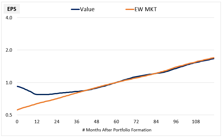
- The market re-rates value stocks when it anticipates this recovery
- P/E expansion occurs before and during EPS stabilization
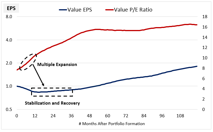
- P/E expansion occurs before and during EPS stabilization
Estimating the valuation disparity
- Clearly, value stocks deserve a valuation discount. Is the market's discount fair or excessive?
- In the long run (in our sample), the value index equilibrated at 60% of the EPS of the EW market index. So the value index should be priced at 60% of the market valuation
- The P/E should have been 9.2x on average, but instead it traded at 7.6x
Comparing current prices to future earnings
- If we calculate E/P using actual (cheaty) forward earnings in year 10, EW market starts at a 19% E/P, value starts at 25%. So the value index is getting earnings for cheaper
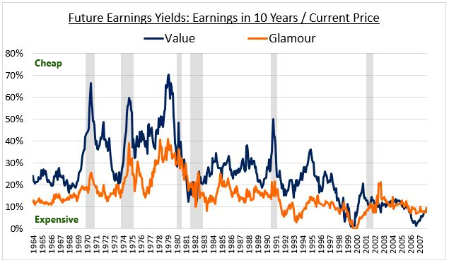
- me: looks like glamour beat value much more often in 2003–2008 than previously (OSAM says this is because of the financial crisis)
- Across the sample, the 10th-year E/P premium for value was 71% (t=22 (!))
Making sense of value's recent performance
- Value had worse 10th-year E/P than glamour in most 10-year periods that overlapped the 2008 financial crisis
- The financial crisis crushed the earnings of value stocks. The re-rating process shouldn't have occurred because value stocks failed to recover
- 5th-year forward E/P graph shows bad 5th-year earnings for value for the 5 years before the financial crisis, but value should be beating growth more recently
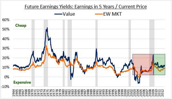
- Value's underperformance doesn't have a definitive explanation. We would point to certain types of hyper-profitable companies (think FAANG) that have dominated the return landscape
- Value stocks today (2018) aren't much cheaper than the market
- The long-term risk to the value factor is not that value companies might suffer periods of extended fundamental weakness, but that the market might arbitrage away the value factor
- me: why? why couldn't companies suffer periods of extended fundamental weakness?
Timing the value factor
- Does value have a higher 1-year return when value is cheaper?
- Yes, with r2 = 0.42
- But dispersion of future returns is very high at normal valuation levels
- Correlation is almost entirely on the short side. Value vs. Market only has an r2 of 0.05
How momentum works: A growth strategy done right
Winners and losers
- Our index invests in the top quintile of stocks by trailing 6-month return
- Like Glamour, the Momentum index has a sawtooth effect where EPS goes up within periods and drops down on rebalancing
Winners vs. Losers:
Winners Losers Difference Total Return 12.6% 7.7% 4.9% Holding EPS Growth 22.5% -20.9% 43.4% Rebalancing EPS Growth -11.1% 27.7% -38.8% Unrebalanced PE Expansion 1.1% 0.8% 0.3% - Winners vs. Losers shows the same pattern as Value vs. Glamour where one gets high holding growth and low rebalancing growth, except in this case the high-holding-growth portfolio wins
Winners vs. Glamour:
Winners Glamour Difference Total Return 12.6% 8.5% 4.0% Holding EPS Growth 22.5% 17.7% 4.8% Rebalancing EPS Growth -11.1% -9.8% -1.3% Unrebalanced PE Expansion 1.1% 0.7% 0.5% - Momentum is doing a better job of identifying growing companies than Glamour. But like Glamour, prices get re-rated downward on rebalances
- Momentum shows stronger holding EPS growth in more concentrated portfolios
Divergence from fair value and momentum's subsequent reversal
- Starting from around one year onward, momentum strategies underperform
- This suggests the momentum index tends to overshoot fair value and then revert
- Momentum portfolios on average started out at a –9% future yield premium (i.e. 9% overvalued), rose to –12% by 12 months later, dropped back down to –9% by 30 months out, and slowly reverted toward 0%
- Even at initial portfolio formation, momentum historically usually had a worse 10th-year forward E/P than the EW market
Momentum as overreaction
- Value is an overreaction to bad fundamentals; momentum is a (timeable) overreaction to recent fundamentals growth
- Both value and momentum are correcting mistakes, but with value, the mistake already happened, and with momentum, the mistake happens after you invest
- This helps explain why value and momentum are complementary: value does poorly when prices are moving away from fair value, but momentum does well
Momentum factor timing
- There's no relationship between the relative starting valuation of UMD and subsequent one year return (r ~= 0)
- So you can't time the momentum factor using the value spread
AQR: 2023 Capital Market Assumptions for Major Asset Classes finance
Table of 5–10 year Geometric mean return (CAGR)
- Geometric mean return (CAGR)
- Real = return after inflation
- Excess = return minus RF, which is the nominal return any investor will get if they currency hedge
| Real | Excess | |
|---|---|---|
| US equities | 4.2 | 2.7 |
| int'l developed equities | 4.8 | 4.6 |
| emerging equities | 6.0 | 4.4 |
| US high yield credit | 3.2 | 1.7 |
| US investment grade | 2.6 | 1.1 |
| US 10-year Treasuries | 1.3 | -0.3 |
| int'l dev 10Y Treasuries | 0.9 | 0.3 |
| US cash | 1.6 | |
| global 60/40 | 3.0 | |
| commodities | 4.6 | |
| value-tilted long-only | 0.5 | |
| multi-factor long-only | 1 |
Market-neutral style premia
| Sharpe | |
|---|---|
| single style, single asset class | 0.2–0.3 |
| diversified composite | 0.7–0.8 |
Updated estimates
- For methodology, see 2022 Updated estimates
- The 2023 text is basically identical to the 2022 text
Emerging market equities—assessing the strategic case
- Forward-looking expected return for emerging – US is >3%, its highest in decades
- Emerging markets have a bigger value spread than developed markets (97th percentile vs. 92nd percentile)
Performance of institutional managers according to eVestment data (gross of fees) 2012 to 2022:
systematic discretionary US large cap 0.06 0.03 emerging large cap 0.45 0.19 - Emerging markets are exposed to greater currency risk + a carry premium
Waiting for the axe to fall? Rising cash rates and market risk premia
- Bond yields went up, but equities did not comparably reprice, so bonds look relatively better than last year
- Negative yield curve implies a negative excess return for long-term Treasuries
Geczy & Samonov: Two Centuries of Multi-Asset Momentum (Equities, Bonds, Currencies, Commodities, Sectors and Stocks) finance factors momentum
https://papers.ssrn.com/sol3/papers.cfm?abstract_id=2607730
- Combined momentum over two centuries has a t-stat of 12.7
- me: The p-value is too small to calculate. SciPy can only find p-values as small as t=8 -> p=1e-15
- This is a strategy that combines cross-asset and within-asset momentum for country equities, bonds, currencies, commodities, sectors, and stocks
Table of results
Momentum Strategy T-Stat Monthly Return country equity 10.6 0.88% cross-asset class 10.2 0.45% currencies 9.6 0.51% country-neutral sectors 6.6 0.36% US stocks 6.0 0.51% inverse commodities 5.5 0.45% global bonds 2.3 0.13%
AQR: Trend-Following: Why Now? A Macro Perspective finance trend macro
https://www.aqr.com/Insights/Research/White-Papers/Trend-Following-Why-Now-A-Macro-Perspective Trend Following Why Now A Macro Perspective.pdf
- Trendfollowing failed in the 2010s and is working now due to macroeconomic drivers that were muted in the 2010s (see [2020-05-01 Fri] AQR: You Can't Always Trend When You Want (2020))
- We expect these drivers to be stronger in the future, making trendfollowing work better
Trend-following's strong track record is undiminished
- The SG Trend Index, established in 2000, beat 60/40 both absolutely and risk-adjusted from 2000–2020, but underperformed 2010–2019
- SG Trend Index maintained a low/negative correlation over the full period
- In 2010s, markets displayed unusually small moves, which coincided with a stable global economy and few (if any) major crises
Anomalous forces helped caused trend-following's lean 2010s
- Backdrop:
- benign macroeconomic shocks
- soft growth and low inflation
- central bank policy constrained by low long-duration bond yields
- Central banks suppressed market volatility, preventing price trends
- Trendfollowing strategies capture the tendency of markets to gradually incorporate new information
- 2010s had unusually low GDP growth volatility and few large market moves
- Central banks could suppress economic volatility for two reasons:
- They could add monetary stimulus without risking high inflation
- Bond yields <3% would normally be highly stimulative, but they weren't in the 2010s because "r-star"—the real policy rate consistent with a neutral policy stance—was very low
The return of macro volatility and major market moves
- Trend-following has performed well in the more volatile macro environment of 2022
- Several key challenges make it improbable that economic conditions will return to 2010s levels within the next couple years
- Inflation would have to reduce. Historically, high inflation takes years to subside
- Recent monetary tightening (raising rates) will likely decrease growth in 2023, with many forecasters projecting recession
- Central banks appear to face difficult tradeoffs between growth/employment and inflation, so they are less able to suppress market moves
Trend-following is back
- Some are worried that they're late to the party. We believe there is a reasonable chance that strong returns will continue
- Historically, after 12 months of strong performance trend-following performs about average over the following 12 months (there is no 12-month mean reversion)
AQR: Demystifying Illiquid Assets: Expected Returns for Private Equity (2019) finance alternatives assetallocation
- Leveraged small value is a better benchmark for PE than a large-cap index
- IRRs (internal rates of return) can be especially misleading if they are compared against the time-weighted returns used for public market indexes
- Smoothed returns of PE understate the true economic risk
- Richening valuations of PE may be a headwind for future returns
Theory
- If PE has greater exposure to certain risk factors, then it should earn a compensatory higher return
- Based on economic intuition and empirical evidence, we expect PE to have higher exposure to financial leverage (equity risk), illiquidity premium, size, and value
- PE firms have 2–4x the debt/equity ratios as public companies (avg 100–200% vs. 50%)
- Private Equity's Diversification Illusion (Welch 2017) showed how traditional methods of valuation understate PE's risk. They report equity beta < 1, but a beta of 1.2–1.5 is more realistic
- In principle, a 5–10 year lockup justifies a 4–6% illiquidity premium. But data suggests that the illiquidity premium is largely offset by investor willingness to pay for return-smoothing
- Investors might overpay for PE if they attribute its higher returns to alpha instead of equity risk premium
- Evidence on private real estate supports this: private real estate has underperformed REITs (Ilmanen, Chandra, and McQuinn (2019) and Ang, Nabar, and Wald (2013)
- PE historically had small cap and value tilts. Value tilt has disappeared more recently
Historical performance
- PE beat large-caps by 2.3% and 1.2x-leveraged small-caps by 0.7%, and lost to small-cap value by 1.6%
- Corroborated by Stafford (2017), "Replicating Private Equity with Value Investing, Homemade Leverage, and Hold-to-Maturity Accounting"
- IRRs are too gameable. Public market equivalent (PME) is a better metric of relative performance
- PME compares PE fund to a comparable public market fund where the same amounts of money were invested at the same times
- PE/PME had large EBITDA/EV valuation gaps 1998–2006, but basically no valuation gap 2006–2018. PE outperformance has shrunk, but still positive
- Some studies have found continued PE outperformance after 2006; others found no outperformance
Greg Nuckols: The Complete Strength Training Guide fitness
Intermediate training
- Almost always do main lifts at 70% to 90% of max intensity
- Train low volume on main lifts to avoid overuse injuries. Stay 1–2 reps shy of failure
- Do high volume accessory work: 4–6 sets of 6–15 reps
- Train each muscle group 2–3 times per week
- Bulk/cut phases build muscle faster than maintaining constant body fat
- Move half a pound per week from 10–15% up to 20%
- me: That's basically 12 weeks of pushing PRs, then deload and 12 weeks of lighter work while cutting
- me: Half a pound probably isn't enough to make me hungry. I lost half a pound per week by accident during the sandwich era
- Move half a pound per week from 10–15% up to 20%
- Bodybuilding-style training has much lower injury rate than powerlifting-style
me: My thoughts me
- My current program is pretty good, except that I should do higher reps on accessory work (chins, dips, DB bench, face pulls), although I kinda already knew that and I just don't like doing high reps
- For chins and dips, switch from 5 reps to 8 reps
What's Wrong with Social Science: Reflections After Reading 2578 Papers
https://fantasticanachronism.com/2020/09/11/whats-wrong-with-social-science-and-how-to-fix-it/
- Based on predicted replications from a sample of 3000 papers in DARPA's Replication Markets program
- 175 of the papers will actually be replicated
- Studies that replicate are cited at the same rate as studies that do not
- There is no correlation between a journal's reputation and predicted replication rate
- Economics papers have the best predicted replication rates; sociology and education come next. Marketing, management, and cognitive psychology look the worst
- People have been writing about the replication crisis since the 1950's, eg Sterling (1959)
- I believe the most valuable activity in metascience is not replication or open science initiatives but political lobbying:
- Earmark 60% of funding for pre-registered papers
- Earmark 10% of funding for replications
- Lower significance threshold to .005
- The median researcher is a hack and the median paper should not exist
Gwern: What Is the Morning Writing Effect? self_optimization writing
https://www.gwern.net/Morning-writing
- Confidence: Possible
- Many financially independent authors write first thing in the morning for 3–4 hours, and spend the rest of the day on less-demanding activities
- But systematic survey evidence is limited
Some reasons why morning writing might appear better
- Ecological fallacy: at the population level, being a night owl is correlated with creativity, but the very best writers tend to be larks
- Top early-morning writers don't report major struggles with focusing in the morning, which suggests that they're larks, and night owls might not perform well if they force themselves to write in the morning
- People are bad at scheduling, and if they intend to write later in the day, they won't get around to it
- The day uses up some sort of 'willpower' or 'creativity'
- Sleep appears involved in unconscious processes of creativity. You wake up primed to work, and by instead puttering around making breakfast, you dissipate the potential
- Or perhaps there is something special about the liminal half-asleep state
AQR: Time Series Momentum (2012) trend
http://docs.lhpedersen.com/TimeSeriesMomentum.pdf
- Speculators profit from TMOM at the expense of hedgers. Speculators follow trends, hedgers bet against trends
- Determined using data from CFTC looking at traders' self-classifications as non-commercial (speculator) or commercial (hedger). See section 2.2 "Positions of traders"
Vogel: Long-Only Value Investing: Does Size Matter? value
https://papers.ssrn.com/sol3/papers.cfm?abstract_id=4078256
- Across four value metrics, long-only small-cap value VW and EW perform about the same as large-cap value EW
- True 1973–2020 in both US and international and for various construction methodologies
- Large-cap value VW performs worse, possibly driven by mega-cap outliers
- Long/short small-cap value still beats long/short large-cap value
AQR: 2015 Capital Market Assumptions for Major Asset Classes
(only taking notes on the style premia part)
Long/short alternative style premia
- We look at value, momentum, carry, and defensive
- Current valuations aren't useful because holdings can change rapidly
- me: They don't really say anything helpful
AQR: 2022 Capital Market Assumptions for Major Asset Classes finance
Table of 5–10 year expected returns
- Geometric mean return (CAGR)
- Real = return after inflation
- Excess = return minus RF, which is the nominal return any investor will get if they currency hedge
| Real | Excess | |
|---|---|---|
| US equities | 3.6 | 5.1 |
| int'l developed equities | 4.3 | 5.8 |
| emerging market equities | 5.3 | 4.4 |
| US high yield credit | 0.3 | 1.9 |
| US investment grade | 0.4 | 1.9 |
| US 10-year Treasuries | -0.8 | 0.8 |
| int'l dev 10Y Treasuries | -0.6 | 0.9 |
| US cash | -1.6 | |
| global 60/40 | 1.9 | |
| commodities | 1.4 | 3 |
| value-tilted long-only | 0.5 | |
| multi-factor long-only | 1 |
Market-neutral style premia
| Sharpe | |
|---|---|
| single style, single asset class | 0.2–0.3 |
| diversified composite | 0.7–0.8 |
Updated estimates
- 50% chance that 10-year realized equity returns will be off by >3% per year
Equities
- Earnings-based approach: E[r] = Shiller E/P * payout ratio + EPS growth
- Payout-based approach: E[r] = dividend yield + buyback yield + avg(earnings growth, GDP growth)
- Final estimate is an average of earnings-based and payout-based
- We assume no mean reversion in valuations
Bonds
- Yield + capital gains from rolldown
- For non-government bonds (IG and HY), apply a 50% haircut to spreads to represent expected defaults + downgrading bias + bad-selling practices
- Historical credit risk premium is about half the spread
- "bad-selling" = selling bonds that get downgraded and no longer meet index criteria
- For IG and HY, correct for convexity and variance drag
Commodities
- We find no statistically significant medium-term predictability, so our estimate is just the historical long-run average
Alternative risk premia
- Estimates are net of fees
- See 2015 report for methodology, which we believe are plausible and conservative
- We don't generally like factor timing, but the current extreme cheapness of value warrants an overweight
Katja Grace: Anthropic Principles philosophy
https://meteuphoric.com/anthropic-principles/
- Self Sampling Assumption (SSA): You are more likely to be in worlds where a greater proportion of people are like you
- Self Indication Assumption (SIA): You are more likely to be in worlds where there are a greater number of people like you
- me: Article includes brief pros/cons of each theory
Bye: How Long Can People Usefully Work? self_optimization
https://www.lesswrong.com/posts/c8EeJtqnsKyXdLtc5/how-long-can-people-usefully-work
- There is no good research on how long people can usefully work
- We don't know how long people can usefully work
Ranadive: The Pyramid Principle writing
https://medium.com/lessons-from-mckinsey/the-pyramid-principle-f0885dd3c5c7
- The Pyramid Principle is used by McKinsey in making presentations to executives
- It's useful any time you want to persuade someone
Start with the answer first
- Executives want to know what to do. Give them the answer first so you don't waste their time. You can explain the reasoning afterward
Group and summarize your supporting arguments
- Ideas should form a pyramid: key point > supporting arguments > sub-supporting arguments
- Aim for 3 points at each level of the pyramid
Logically order your supporting ideas
- A few ways of ordering ideas:
- Time order: sequence of events with cause-effect relationship
- Structural order: thought + supporting ideas
- Importance order: most to least important
Carlisle: ROIC and Reversion to the Mean finance factors value
https://greenbackd.com/2010/04/21/roic-and-reversion-to-the-mean-part-1/ https://greenbackd.com/2010/04/22/roic-and-reversion-to-the-mean-part-2/ https://greenbackd.com/2010/04/27/roic-and-reversion-to-the-mean-part-3/
- Top-20% ROIC companies had a 64% chance of being in the top 40% 10 years later, and a 41% chance of being in the top 20%
- Bottom-20% ROIC companies showed similar persistence
- But of the companies that start and end in the top quintile, less than half stay in the top quintile the whole time
- Certain industries (biotech, software) are overrepresented in both the bottom and the top quartile
- Breaking ROIC into earnings/sales (margin) and sales/ROIC (inventory turnover), persistent high-ROIC companies had more of an advantage on margin than on turnover, but it wasn't a strong effect (2.4x median vs. 1.9x)
McCluskey: The Future of Earning to Give (2019) career causepri
http://www.bayesianinvestor.com/blog/index.php/2019/10/13/the-future-of-earning-to-give/
- Are the 2–3 big EA grantmakers going to find all the best opportunities? I find this less plausible than that the 2–3 best VCs will fund all the good startups
- Even if the best current opportunities get funded, in the long term we will need more funding for bigger, harder causes
- It would be an odd coincidence if the skills needed by EA orgs heavily overlap with the skills of EAs
Sumner: It Didn't Begin with COVID econ
https://www.econlib.org/it-didnt-begin-with-covid/
- People often criticize the US government for overreacting to COVID
- But the US government has overreacted to lots of things to a much greater extent
- There have only been two airline deaths in the past 11 years, but people are still required to wear seatbelts. And we're not required to wear seatbelts on buses, trains, or boats
- I find the TSA to be 10 times more annoying than COVID regulations
- COVID regulations might be too severe, but at least COVID is a meaningful problem that has killed 800,000 Americans, unlike airline crashes or terrorism
Hamming: You and Your Research (1993)
https://www.cs.utexas.edu/users/dahlin/bookshelf/hamming.html
- You cannot do important work if your problem area is not important and tractable
- Great scientists spend a lot of time examining the important problems in their field
- Many keep a list of the 10 or 20 most important problems. Then, when they learn something that seems relevant, they are prepared to work on the corresponding problem
- People who keep their office doors open get distracted more easily, but people who keep their doors closed tend not to know what to work on
- Most great scientists work hard
Personal traits
- Successful people look more places, they work harder, they think longer than less successful people
- The highest quality work comes from people who are emotionally committed to their work
- Perhaps the best mathematician I know produced good work, but not top quality, because he didn't care deeply about his work
- Courage—willingness to attack difficult problems
- Ability to tolerate ambiguity
- It is a fine balance between believing what you learn and at the same time doubting things
- You need to think about things from many angles, put "hooks" in them. Connect them in many ways to what you already know so you can later retrieve them in unusual situations
- Most outsiders are kooks, but the best insights often come from them. I have no simple answer except do not dismiss outsiders too abruptly
Vision
- You need a vision of who you are and where your field is going
- Some of the greatest work was done under unfavorable conditions
- What most people believe is the best working conditions for them is seldom, if ever, true
- The supposedly ideal working conditions of the Institute for Advanced Study has ruined more good people than it has helped
Selling
- You must present your results so that others will listen to you
- Lots of good work has been lost because of poor presentation, only to be rediscovered later by others
Is it worth the effort?
- Those who have done great things generally report, privately, that it is better than wine, the opposite sex, and song put together
- It is in the struggle and not the success that the real gains appear
Sam Bankman-Fried fireside chat causepri
https://www.youtube.com/watch?v=--tV8U3BbJk
- I think Cause X is more likely than most EAs think it is
- Lots of uncertainty about the best cause. Far future appears overwhelmingly important in EV. But unclear what to do about it. My biggest priorities:
- Biorisk / pandemic preparedness
- AI safety
- Politics
- The obvious, naive "change the world" approach is to go into politics. But it's likely correct
- I don't think it's true that you can only do 20 productive hours of work a week. If anything, time working is super-linearly valuable because it takes time to build context. My first 20 hours are useless
- If you're earning to give, you should go for straight EV, which means high risk. If your goal has a >30% chance of success, it's probably not ambitious enough
- Bottleneck for direct work is starting things. There's funding, there's people willing to join things that have already started
- Don't go to grad school. I cannot emphasize this enough. You can learn much better outside of academia
Swedroe: Is There a Replication Crisis in Finance? (2021) finance factors
https://alphaarchitect.com/2021/03/23/is-there-a-replication-crisis-in-finance/
Summary of a paper with the same title
- Factors clustered into 13 themes: Accruals (-), Debt Issuance (-), Investment (-), Leverage (-), Low Risk, Momentum, Profit Growth, Profitability, Quality, Seasonality, Size (-), Skewness (-), Value
- A (-) indicates a reverse factor
- In Bayesian model, 10 of 13 themes had at least 75% of factors replicate, the exceptions being Seasonality, Leverage, and Size
- An efficient-frontier portfolio included 10 of the 13 themes, the exceptions being Profitability, Investment, and Size
- Value factors became stronger when controlling for other themes (especially Momentum, Quality, Leverage)
Me: Do AlphaArchitect funds capture these 13 factor themes?
- QVAL includes mostly Value, but also Profitability, Profit Growth, Quality, Low Risk, and Accruals
- QMOM includes mostly Momentum, but also Low Risk (albeit a different interpretation) and Seasonality
- They sorta capture Size by equal-weighting
- They don't capture Debt Issuance, Investment, or Skewness
- but Investment is highly correlated with Value
The Cross-Section of Speculator Skill: Evidence from Day Trading (2013) finance
https://faculty.haas.berkeley.edu/odean/papers/Day Traders/The Cross-Section of Speculator Skill.pdf
- We find large cross-sectional differences in the before- and after-fee returns earned by day traders in Taiwan from 1992 to 2006
- Top-ranked traders in year n go on in year n+1 to earn before-fee (after-fee) returns of 0.61% (0.38%) per day
- Less than 1% of the day trader population is able to reliably earn positive abnormal returns net of fees
Introduction
- Prior research shows that even before fees, individual investors tend to buy stocks that underperform the market
- Prior research finds variables that reliably predict performance: IQ, cognitive abilities, geography, portfolio concentration, age, past performance. But even skilled stock pickers in these studies are unable to beat transaction costs
- Most prior studies examine all individual investors, most of whom trade infrequently, and use data from only a single broker
- We look at all transaction data for the Taiwan stock market 1992–2006
- Day traders account for 17% of volume
- This percentage is remarkably stable over time
- Day traders account for 17% of volume
- Day trading: The purchase and sale of a stock in the same day
- 20% of day traders earned positive abnormal net returns, and about 1% were able to predictably profit
- Profitable day traders earn more in small-cap and high-vol stocks, and in periods around earnings announcements
- Profitable day traders do not appear to make money by providing liquidity
- Aside from past performance, the best predictor of future performance is concentrating in a small number of stocks
- This suggests that successful day traders gain an information advantage by carefully studying a few stocks
Results
Active day traders
- Top 500 day traders ranked by prior year performance have a future net alpha of 0.38% (t=61)
- me: This is a lot less significant than it sounds because returns are not normally distributed
Sources of profits
Are day traders informed?
Earnings announcements
- Top 500 investors earn 0.66% daily alpha in the 5-day window around earnings announcements, and 0.59% daily alpha all other times (t-stat of difference = 2.8)
- me: They use this to conclude that top day traders earn stronger returns during periods of high information asymmetry, which does appear true, but the effect is pretty small
Hard-to-value stocks
- Top traders earn higher profits in small-caps (t=15)
- The top 10,000 traders earn higher profits in high-vol stocks (t=11), but the top 500 do not (t=1.1)
AlphaArchitect: The World's Longest Multi-Asset Momentum Backtest (2018)
https://alphaarchitect.com/2018/04/24/the-worlds-longest-multi-asset-momentum-investing-backtest/
- A summary of Two Centuries of Multi-Asset Momentum (Equities, Bonds, Currencies, Commodities, Sectors and Stocks)
- Momentum factor had negative performance for four decades from 1840 to 1880 in equities and currencies, and from 1850 to 1890 in commodities
- Although combined multi-asset momentum only had one decade of negative performance (1820)
Two Quants: Takeaways from "The Man who Solved the Market" finance
https://twoquants.com/the-man-who-solved-the-market-part-1/ https://twoquants.com/the-man-who-solved-the-market-part-2/
- Medallion started out mainly doing short-term trendfollowing
- "As Renaissance staffers struggled to improve their model throughout the 1980s, they kept hearing about Richard Dennis’s successes."
- When Morgan Stanley would put on a big trade for a client, it would hedge with a similar asset (e.g., if a large seller wants to sell Coke, Morgan Stanley will buy Coke from them while selling Pepsi). Medallion would profit off this by looking for big block trades and then betting on mean reversion in price differences
- They looked for strategies with p < 0.01
Feynman: Take the world from another point of view (video)
https://www.youtube.com/watch?v=mvqwm6RbxcQ
- One time I was struggling with a problem for years and I thought, there has to be a simple answer. So I took a step back and tapped on it a little, and then I found the answer. But I've tried doing that other times and it hasn't worked
- I've tried to figure out under what conditions I'm most likely to have insights, but I can't find anything. The conditions seem random
Matheny: Reducing the Risk of Human Extinction (2007) causepri xrisk
http://wilsonweb.physics.harvard.edu/pmpmta/Mahoney_extinction.pdf
- The probability of extinction this century may be very low, but the expected value of preventing it could be high
Humanity's life expectancy
- We face near risks (nuclear war, asteroids), risks of as yet undeveloped technology (nanotech, AI), and long-term risks (sun expansion)
- Homo sapiens has existed 200K years; homo erectus 2M years; median species lasts 2M years
- Anthropic doomsday argument suggests humanity won't last much longer
Estimating the near-term probability of extinction
- Several people have estimated the probability of extinction at 25-50% this century
Reducing extinction risk
- NASA spends $4M/year on monitoring asteroids and comets; $1.7B is spent on climate change
- Bioterrorism might be the most severe risk; US spends $5B/year on biodefense
- Unclear risks from high-energy physics experiments; Posner (2004) recommended withdrawing federal support for these experiments
- We have bunkers for government leaders and seed storage facilities, but no way to shelter large numbers of people during a potential extinction event
- As few as 100 people could repopulate earth. The Americas and Polynesia were originally populated by fewer than 100 founders
Discounting
- Discounting has been justified based on time preference, consumption growth, uncertainty about future existence, and opportunity costs. None of these justifications applies to the benefits of delaying human extinction
- Justification for time preference is typically descriptive. But observed time preference might only apply to instrumental goods, like money, whose value decays over time
- It would be difficult to design an experiment in which time preference for an intrinsic good, like happiness, can be separated from forms of non-pure discounting
- We should reject time discounting just as we reject spatial discounting
- It is better to invest in stocks rather than x-risk if: ROC is exogenous to the rate of social savings; ROC is higher than the rate of technological change in extinction countermeasures; marginal cost-effectiveness of countermeasures does not decrease faster than ROC
- Exogeneity is false
- Spending on countermeasures tends to accelerate learning
- If x-risk decreases after space colonization, then we might be living in a particularly influential time
Example: the cost-effectiveness of reducing extinction risks from asteroids
- Suppose, absent extinction risks, humanity survives as long as homo erectus did, at a population of 10 billion. That gives us 1.6 million years remaining, and 1.6e16 life-years
- 1 in a million chance of extinction-level asteroid impact this century
- A system to detect all near-earth asteroids would cost $300M to $2B, and a system to deflect asteroids would cost $1B to $20B to develop
- Assume $20B to run an asteroid deflection program, and a 50% probability of success
- Expected cost is $2.50 per life-year. This is far more cost-effective than many programs we currently fund
Discounting revisited
- Although the usual justifications for discounting do not apply to extinction, we might conclude that working on human extinction is cost-effective even if we accept discounting
- Using Weitzman (2001)'s gamma discounting, asteroid deflection cost $140 per life-year. At a 1% constant discount, it cost $40,000
AQR: Is Systematic Value Investing Dead? finance value
https://www.aqr.com/Insights/Research/Journal-Article/Is-Systematic-Value-Investing-Dead PDF PDF (2021 edition)
Framework
- We define fundamental value as the residual income valuation:
\(F_t = B_t + \displaystyle\frac{E[X_{t+1} - r B_t]}{1 + r} + \frac{E[X_{t+2} - r B_{t+1}]}{(1 + r)^2}\)
- where B is book value, X is forecasted earnings, r is expected return (a combination of risk-free rate, assumed 3% equity premium, and beta of the stock in question)
- That is, fundamental value is current book value plus the next two years' expected earnings in excess of the return on equity
- If we use infinity years instead of two, this is equivalent to the discounted dividend model
Do 'fundamentals' still matter for stock returns?
- Value investing works either by prices reverting to fundamentals, or by buying cash flow for cheap. But the latter is not typical
- If fundamentals converge to price, or if the value spread widens, then value will underperform
- One way to assess whether fundamentals help value investors is to cheat and use future earnings expectations: in year N, take analyst forecasts of earnings made in year N+1
- This strategy performed very well in general, but performed poorly in the dot-com era and for the past few years
- me: "poorly" means Sharpe ~2, vs. average Sharpe ~6
- We decompose returns into (1) dividend + (2) multiple expansion + (3) change in fundamentals
Table 4 regression
- We run a regression predicting stock return based on valuation \(\log(\displaystyle\frac{F_t}{P_t})\) and change in fundamentals \(\log(\frac{F_{t+1}}{F_t})\) (where \(F_t\) is defined above). See Table 4
- Controlling for change in fundamentals, cheap companies outperformed expensive companies every year but 2000. But was very close to 0 in 1999, 2018, and 2019
- me: It makes sense that it would almost always be positive, since cheap company underperformance is driven by worsening fundamentals. I don't think this tells us anything about the performance of value vs. growth
- me: 2007–2019, average return attributable to change in fundamentals was 0.42. Over prior period (1987–2006), average was 0.55. Lower, but only a little.
- This is a much smaller difference than in the RAFI paper. Presumably, most of the recent weak performance in value fundamentals is accounted for in the two-year earnings forecasts
- Also the RAFI paper was looking at explaining value factor performance, and this paper is explaining individual stock performance
- Difference between samples is significant at p<0.0002
- Paper looks at this visually in Figure 7
- Interestingly, explanatory power of valuation was far higher 2001–2002 than any other time since 1987
- This is a much smaller difference than in the RAFI paper. Presumably, most of the recent weak performance in value fundamentals is accounted for in the two-year earnings forecasts
Table 5 regression
- We run a regression predicting stock return on dividend yield, multiple expansion, and change in fundamentals, "holding \(\log \left( \displaystyle\frac{F_t}{P_t} \right)\) fixed" (whatever that means): \(\log(R_t) = \log \left(1 + \displaystyle\frac{D_{t+1}}{P_{t+1}} \right) + \log \left(\displaystyle\frac{P_{t+1}/F_{t+1}}{P_t/F_t} \right) + \log \left(\displaystyle\frac{F_{t+1}}{F_t} \right)\)
- me: Note that the Table 4 regression only explains about 30% of the variation in returns, while this regression (by definition) explains 100%
- me: 2007–2019, average return attributable to change in fundamentals was –24%. 1987–2006, average was –27%. Insignificant difference (p=0.17)
- Return attributable to yield was consistently small (0% to 2%), but lower in the 2007–2019 period
- me: Table 5 shows that valuation (\(\log(\frac{F_t}{P_t})\)) had positive predictive power every year 2012–2017, seems to contradict that the value factor had negative return?
- The periods of weakest performance for value (1990, 1999, 2018, 2019) saw both multiple contraction and weak fundamental mean reversion, but mostly driven by the former
- > Fundamentals do matter for stock returns, but there are periods where stock prices become less connected with fundamental information, and in such periods value strategies underperform. This has happened before, is happening now, and will likely happen again. However, absent a crystal ball allowing an investor to know ahead of time if the market is less in tune with fundamentals, the implication for value strategies is not clear.
Exhibit 9
- me (2022-12-19): Exhibit 9, column 8 is what we want: change in fundamentals attributable to current valuation (as F/P). 1987–2006 had an average of –0.27 and 2007–2020 had an average of –0.23. That means value is doing better than before (high fundamental/price ratio predicts worse fundamentals growth, but less worse). A coefficient closer to 0 means valuation is worse at predicting fundamentals growth. This doesn't explain anything. What we want is (implicit) predicted fundamentals growth vs. actual fundamentals growth
[ ]We should be able to convert the valuation into a prediction about fundamentals growth (although it's dependent on discount rate)- 2026-02-06: idk why I said this doesn't explain anything. I think this shows that valuation has gotten worse at predicting fundamentals growth
- me: t-stats under \(R_{t,t+12}\) show that F/P ratio can have very strong positive or negative predictive power, with t-stats like 16.7, 11.7, -7.3, and -7.0. This basically falsifies a model where value stocks have some random but positive-EV return, and supports the existence of a unified value factor that explains the cross-section of returns
Summers & Zeckhauser: Policymaking for Posterity (2008) causepri
- Contrary to conventional prescriptions, the greater wealth of future generations may strengthen the case for preserving the environment
- Lower discount rates should be applied to the far future
- Extinction does not merit infinite negative utility
- Given learning, greater uncertainty about damages could either increase or decrease the optimal level of x-risk reduction
- Policies for posterity should anticipate behaviors of other actors and of future generations, which could change in surprising ways
I. Introduction
- Two widely held conclusions in the literature:
- Market discount rates are not the right indicator for altruistic projects
- Market discount rates are much higher than society's true discount rate
- This implies that altruistic projects should weight the future more highly
- Our goal is not to determine the social discount rate, but to identify a range of considerations on how to allocate resources over the long run
- Section II: Results from behavioral psychology generally suggest giving more weight to the future than a standard discounting approach would
- Section III: The pure uncertainty case for giving greater weight to the future (e.g., Weitzman) is less compelling than many have suggested
- Section IV: Any choice we make could change the choices of other actors and future generations
II. Policy for posterity given certainty
- Fundamental discounting equation: \(\rho = \delta + \eta g\)
- There are several issues that do not fit into this standard approach
Global population issues
- Fundamental discounting equation ignores population size. We believe the weight of a generation should depend on its size, probably linearly
- Can adjust by subtracting the rate of population growth from the social discount rate (population growth is effectively a negative discount)
Consequences of income growth
- According to one argument, future people will be far richer, so spending money now to help the future is effectively reverse wealth distribution
- The standard discounting approach only applies when trading off current vs. future consumption. For climate change, the benefit of actions taken today should be measured in terms of the future's willingness to pay, which rises with income
Characterizing altruism
- When considering the possibility of extinction, it seems like we should not discount the future at all, or at least should not use exponential discounting
- A 10% chance of preventing a comet impact 400 years from now seems better than a 1% chance of preventing a comet impact 100 years from now
- If generations continue infinitely, then a loss that continues forever matters infinitely more than any benefit today
- We think it is essential to have a system where a finite loss to each generation over an infinite future counts far less than infinity
- Due to scope insensitivity, asking people to value a cost to a single generation at a far future date may lead to a similar valuation to asking about that same cost across all generations starting from that future date
Reference points, loss aversion, and errors of commission
- Some argue that we have a special obligation to preserve the environment because it was bequeathed to us by nature
- There are three strong elements to this argument: reference points, loss aversion, and errors of commission
- Prospect Theory: people treat losses from some reference point as more consequential than gains
- Reducing per-capita income to mitigate climate change hurts people more than reducing income growth
- Improving the environment requires purposeful action. But people usually believe it is more important to mitigate their own acts of commission, rather than omission (e.g., they don't litter, but they don't pick up other people's litter)
- Therefore, we should give greater weight to harms done by our actions than to harms from external events
Summary
- These considerations all make the case for giving more weight to the distant future than the fundamental discounting equation suggests
III. Policy for posterity given uncertainty
- Weitzman has argued that uncertainty strengthens the argument for prioritizing the future
- Here we suggest that the effects of uncertainty are less clear cut, due to two issues:
- Proper modeling of low-probability catastrophic events
- Learning on the timing of mitigation policies
Valuing low-probability catastrophic losses due to climate change
- To simplify, suppose only the current generation has to decide between consumption and helping the far future
- We must decide whether to rely on how most people behave or on rational decision theory, because the answers can be far different
- Behavioral approach says we should probably not act to reduce low-probability risks
- For climate change, we believe society should follow rational decision theory rather than behavioral propensities
- We assume there can only be two outcomes, normal or cataclysm (e.g., extinction)
- Societal cataclysms can be considered similarly to how individuals consider personal cataclysms
- Suppose Alice has a 1% chance of dying next week, and this can be reduced to 0% for a price. How much should she pay?
- Let U(w,e) be a VNM utility function of wealth and existence (1=alive, 0=dead)
- Solve for x in \(0.99 U(w, 1) + 0.01 U(w, 0) = U((1-x)w, 1)\), where x is the maximum fraction of wealth she's willing to spend (wealth includes human capital)
- Most people would be willing to spend more than 1% but less than 90%. If \(U(w,1) = 1\) and \(U(w,0) = 0\), then \(U(0.1 w,1) < 0.99\)
- \(U(w,0) = -\infty\) seems unreasonable, but this is what Weitzman (2008) assumes
Uncertainty and learning and the timing of climate change mitigation
- Some argue that uncertainty means we should act now to mitigate climate change b/c there's more downside risk. Others argue that uncertainty means we should wait and learn more
- Which effect dominates depends on parameter values
- We built a model where you can spend to mitigate climate change in period 1 or period 2, and get some learning between periods, and mitigations have increasing marginal costs with respect to emissions. Increasing uncertainty can relatively favor spending in period 1 or period 2, depending on the learning rate and on the rate of increasing marginal costs
- Second period has higher emissions, so emissions need to reduce by more, giving a higher marginal cost to reduce emissions
- If cost to reduce emissions by r is \(c(r) = r^a\) for a > 1, then increasing uncertainty relatively favors spending later when a < 2, and relatively favors spending now when a > 2. Cutoff at a = 2
Risk aversion
- In the above model, increasing marginal costs were not due to risk aversion, but to increasing real costs of reducing emissions
- Assume risk aversion of costs. If the disutility of costs follows a power function, then we can use the same model but with a different (larger) marginal cost parameter. This pushes the cutoff to a < 2, so it's more likely that uncertainty relatively favors spending now
- If instead we assume risk aversion on damages, then more uncertainty pushes toward spending now
Geoengineering
- Most discussion focuses on curbing emissions (mitigation), but we could also fix climate change via geoengineering
- Geoengineering is relevant even if it appears to be a bad idea. Suppose geoengineering is as bad as a 20% decrease in global consumption, and there's a 1% chance that climate change will be as bad as 90% decrease in consumption. Then there is a low probability that geoengineering will ultimately look attractive, even though it doesn't today. If feasible, geoengineering puts an upper bound on how bad climate change can get
- Geoengineering may be necessary if the current level of emissions will still result in severely bad outcomes
IV. Reaction function issues
- People whom the policymaker does not control are likely to adjust their behavior in response to changes in policy
Effects on alternative investments
- The attractiveness of a policy depends on the alternatives
- An initiative that is likely to crowd out scientific research should be judged more harshly than an equivalent project that would crowd out only consumption
The intergenerational game
- We would not be pleased to take costly action only to find that future generations slacken their effort in response
- On a standard reaction function analysis, the more we do today, the less will be done tomorrow. See Arrow (1999)
- On the other hand, perhaps good deeds today could set a precedent
- Building off of Schelling (1957): actions framed as noble precedents, and established around bright-line markers, are more likely to stimulate continuing altruism in future generations
International considerations
- Nations that mitigate climate change produce positive externalities, and yield only modest benefits for their own citizens
- Will nations abide by international agreements in the absence of enforcement mechanisms?
- More extensive efforts by a particular nation might encourage reciprocity
Technology
- Cost estimates for major policy changes seem to usually underestimate the actual cost
- But experience in the environmental area shows that the cost of meeting commitments usually falls well below initial estimates (e.g., US sulfur oxide program, LA smog controls, ban on CFCs)
- Cost to reduce emissions, especially in the long term, could easily be 5-10x more expensive or cheaper than expected
V. Conclusion
- We identified four Ds that must be considered
- Our principal conclusion is that analyses that focus on merely one or two of the four Ds will provide an incomplete picture
Discounting
- Standard approach of exponential discounting is problematic because people don't express exponential preferences
- We may value a generation 300 years hence no different than one 100 years hence wrt saving it from a comet collision
Disaster
- Costly efforts to combat climate change are only potentially worthwhile if future disaster threatens
- Unlike Weitzman, we do not accept the existence of infinitely negative outcomes, so we are willing to accept some nonzero probability of catastrophe
Distinction
- We want to take the action with the greatest far-future benefit per unit of cost to us
- Climate change policy must compete with other measures that benefit the far future, such as medical research
Decision analysis
- Greater uncertainty means more expected damages if we delay action, but also greater learning opportunities
Sam Harris: Waking Up books meditation self_optimization
- meditation improves immune system
- if my daughters do not take LSD or psilocybin, I will wonder if they have missed one of the most important rites of passage a human can experience
AQR: Trend Following in Focus (2018) finance trend
https://www.aqr.com/research-archive/research/white-papers/trend-following-in-focus ~/Documents/Reading/Trend Following in FocusSeptember 2018.pdf
Drawdowns are unfortunate but expected
- Recent drawdown for trendfollowing is commensurate with previous large drawdowns
- Trendfollowing delivered positive returns when global equities declined in late 2015
Is trendfollowing over-subscribed? Not likely
- Assets invested in trendfollowing peaked in mid-2008 at $210B, and have declined to $120B
- All systematic hedge fund strategies have $500B AUM, or 17% of all hedge fund assets
- Futures market has grown since 2008, so trendfollowing as a % of futures markets has decreased by more than half
Trendfollowing is a good strategy going through a tough time
- Macro environment has produced few meaningful trends since mid-2016
- Can measure opportunity set for trendfollowers by examining the number and magnitude of trends
- Recent years have seen few such opportunities
- People have a perception of strong trends due to S&P performance [remember, this was written in 2017], but S&P is the exception right now
Conclusion
- The strategy is behaving as expected
- We continue to anchor our expectations for trendfollowing to the long-term evidence
AQR: Commodities for the Long Run (2016) finance alternatives
https://www.aqr.com/Insights/Research/Journal-Article/Commodities-for-the-Long-Run PDF
- We used a novel data set going back to 1877
- Over the long run, commodity futures average returns have been positive
- Return is explained by both spot and carry, but variance in commodity returns are mostly explained by moves in the spot price
- This evidence supports commodities as a potentially attractive asset class in portfolios of stocks and bonds
Introduction
- Return premiums come more from interest rate-adjusted carry than from excess spot returns
- Returns are stronger during backwardation, inflation, and economic expansion
- We find positive returns even in contango when inflation is up or the economy is expanding
Data description and analysis
- "Interest rate-adjusted carry" equals the carry PLUS the risk-free rate, equals the convenience yield
- Can decompose excess return as spot return + carry, or excess of cash spot return + interest rate-adjusted carry. We prefer the latter because both components are economically meaningful
- Paper focuses on excess return over the risk-free rate, not on total return
Data
- 1877 data includes corn, lard, oats, pork, and wheat. Number of commodities in data set stays small until about 1970
- For each month, our backtest held the nearest contract whose delivery month was at least two months away
- Earlier measures appear a little less liquid, but not much
Commodity index returns and aggregate states
- We constructed two portfolios:
- equal-weighted
- long top 1/3, short bottom 1/3 on backwardation
Commodity return properties, 1877–2015
- Performance was better 1946-2015 than 1877-1945, partly due to which commodities were included. Early period was mostly agriculture, later is more diversified
- A Grains Only portfolio performed about the same in both periods
- Actual returns depend on the cost to short, but variation in returns is not explained by shorting cost
- Commodities have had long periods of negative performance. Current period of poor performance is toward the low end, but not unusual
- Worst period was about 1920–1935
Summary statistics 1877–2015
- all returns are excess of RF
| equal-weighted | long/short | bonds | stocks | |
|---|---|---|---|---|
| arithmetic mean | 4.6 | 5.0 | 1.1 | 6.7 |
| geometric mean | 3.1 | 3.4 | 1.0 | 5.4 |
| excess spot return | 2.0 | -26.4 | ||
| interest rate-adjusted carry | 3.8 | 32.6 | ||
| volatility | 17.7 | 18.2 | 5.5 | 17.0 |
| spot volatility | 18.2 | 21.7 | ||
| carry volatility | 5.6 | 13.2 |
Summary statistics 1946–2015
- all returns are excess of RF
| equal-weighted | long/short | bonds | stocks | |
|---|---|---|---|---|
| arithmetic mean | 5.4 | 10.0 | 1.7 | 7.4 |
| geometric mean | 4.5 | 8.7 | 1.5 | 6.5 |
| excess spot return | 1.8 | -22.7 | ||
| interest rate-adjusted carry | 4.3 | 33.4 | ||
| volatility | 14.1 | 17.6 | 7.1 | 14.4 |
| spot volatility | 14.4 | 19.2 | ||
| carry volatility | 3.9 | 9.2 |
Macro performance of commodity portfolios
- We focused on three variables:
- Backwardation/contango of commodity futures market as a whole
- Unexpected inflation, as measured by the one-year change in one-year inflation
- Expansion and recession periods, as estimated by NBER
- These variables all partially explain commodity returns
- Unsurprisingly, carry was higher in backwardation than contango
- Return was still positive in contango
- But spot returns were also lower (t-stat > 3)
- Explanation: backwardation can happen because the market expects spot prices to fall, and the market tends to be right
- Spot return is higher during unexpected inflation, which confirms that commodities hedge inflation
- Commodities' inflation hedging behavior may explain its poor return relative to stocks
- Carry was similar across economic environments, but spot return was much worse in recessions
- Differential between backwardation and contango performance was small during high inflation or expansion, and differential was large during low inflation or recession
- Long/short portfolio did not show statistically significant differences depending on economic or inflationary state, and performance was consistently positive
Commodity index returns and aggregate states
- returns are arithmetic, excess of RF
| return | excess spot | int-adj carry | stdev | bond corr | stock corr | |
|---|---|---|---|---|---|---|
| full | 4.6 | 2.0 | 3.8 | 1.7.7 | -0.07 | 0.23 |
| backwardation | 7.7 | -3.0 | 12.3 | 18.1 | -0.06 | 0.17 |
| contango | 1.8 | 6.5 | -3.9 | 17.4 | -0.07 | 0.29 |
| infl up | 10.1 | 6.8 | 4.7 | 19.1 | -0.05 | 0.21 |
| infl down | -1.0 | -2.8 | 2.9 | 16.1 | -0.08 | 0.27 |
| expansion | 9.2 | 6.1 | 4.2 | 16.6 | -0.08 | 0.20 |
| recession | -7.4 | -8.8 | 2.8 | 19.9 | -0.04 | 0.24 |
| return | excess spot | int-adj carry | stdev | bond corr | stock corr | |
|---|---|---|---|---|---|---|
| full | 5.0 | -26.4 | 32.6 | 18.2 | -0.02 | -0.03 |
| backwardation | 2.0 | -37.6 | 42.6 | 19.1 | -0.05 | -0.05 |
| contango | 7.7 | -16.4 | 23.6 | 17.4 | 0.00 | -0.02 |
| infl up | 6.0 | -27.3 | 34.8 | 19.3 | -0.08 | -0.04 |
| infl down | 4.0 | -25.5 | 30.4 | 17.0 | 0.05 | -0.02 |
| expansion | 4.5 | -27.3 | 33.0 | 17.8 | 0.00 | -0.03 |
| recession | 6.4 | -23.9 | 31.6 | 19.2 | -0.07 | -0.02 |
| bond return | stock return | |
|---|---|---|
| full | 1.1 | 6.7 |
| backwardation | 0.1 | 4.5 |
| contango | 2.1 | 8.7 |
| infl up | 0.2 | 4.1 |
| infl down | 2.1 | 9.3 |
| expansion | 1.1 | 12.3 |
| recession | 1.3 | -7.9 |
Asset allocation and drawdown analysis
- Ex-post MVO allocates 30% stocks, 54% bonds, 16% commodities
- Adding long/short commodities to a 60/40 portfolio improved Sharpe in all four types of economic environments (inflation up/down or expansion/recession)
- Adding equal-weighted commodities to a 60/40 portfolio improved Sharpe in inflation-up and expansionary periods, but decreased Sharpe during inflation-down and recessions. Increased Sharpe overall
- During the 10 largest drawdowns of the 60/40 portfolio, commodities saw varying returns. Commodities often had positive return, but did worse than 60/40 in severe recessions (1929 and 2007)
- Long/short had positive return in 1929 and 2007. Had negative performance in 4/10 periods, but underperformed 60/40 in only one (1937–1938)
Blitz: Strategic Allocation to Premiums in the Equity Market (2011) finance factors
- Investors should include allocations to non-traditional premiums such as size, value, momentum, low vol
- Theoretically optimal strategic allocation to premiums is sizable, even when using highly conservative assumptions regarding their future expected magnitudes
Premiums in the equity market
- Size, value, momentum, low vol premiums
- This is not an exhaustive list, but we use these because data is readily available
- Historical (long-only, large cap) premium sizes in the US from 1963 to 2009, using Ken French data
- For all but size, factor is taken as the top 30%, equal-weighted. Size factor treats 30th to 70th percentiles as small cap
- me: the paper also reports value-weighted, but I'm just writing down the equal-weighted results
- For all but size, factor is taken as the top 30%, equal-weighted. Size factor treats 30th to 70th percentiles as small cap
- Raw long-only portfolios have high correlation to each other because they're all exposed to market beta. But correlations between alphas are lower and sometimes negative
Raw return (excess of RF)
| market | size | value | momentum | low-vol | |
|---|---|---|---|---|---|
| CAGR | 3.9% | 5.7% | 8.3% | 8.8% | 5.9% |
| stdev | 15.6% | 20.0% | 17.4% | 18.5% | 13.3% |
| Sharpe | 0.25 | 0.29 | 0.48 | 0.48 | 0.44 |
CAPM
- me: these can be interpreted as long/short portfolios with the market on the short side
| market | size | value | momentum | low-vol | |
|---|---|---|---|---|---|
| beta | 1 | 1.19 | 0.97 | 1.09 | 0.76 |
| alpha | 0 | 1.1% | 4.6% | 4.6% | 3.0% |
Correlation of CAPM alphas
| market | size | value | momentum | low-vol | |
|---|---|---|---|---|---|
| size | 1 | 0.44 | 0.23 | 0.08 | |
| value | 1 | -0.05 | 0.64 | ||
| momentum | 1 | -0.13 | |||
| low-vol | 1 |
Allocating to premiums
- Size, value, and low-vol have low turnover, but momentum has higher transaction costs
- Will historical premium magnitudes continue in the future? Unclear
Assumptions
- Forward-looking alphas
- market beta: 3%
- size: 0%
- value: 1%
- momentum: 1%
- low-vol: same return as market (implies an alpha of about 0.75%)
- Same vols and correlations as historically
- No short-selling or leverage
- Non-market factors constrained to a max 40% allocation
Resulting allocations
| Market | 1/N | Optimal | |
|---|---|---|---|
| market | 100% | 25% | |
| size | |||
| value | 25% | 23% | |
| momentum | 25% | 40% | |
| low-vol | 25% | 37% |
Predicted performance (excess of RF)
- 1/N portfolio includes market, value, momentum, low-vol (excludes size)
| Market | 1/N | Optimal | |
|---|---|---|---|
| CAGR | 3.0% | 3.5% | 3.7% |
| stdev | 15.6% | 15.3% | 15.4% |
| Sharpe | 0.19 | 0.23 | 0.24 |
Discussion
- Optimal allocation includes factors, in spite of highly conservative performance assumptions
- 1/N is about as good as optimal allocation
Capturing these premiums should be a strategic investment decision
- It's better to make a strategic choice to add factor exposure, rather than trying to get factor exposure accidentally by hiring fund managers with good track records
- Active management does not add value, it's better to get passive factor exposure
- Even if you want active management, it's better to choose in advance what allocation to give to each factor
- This allows you to control overall portfolio risk
Capturing premiums in practice
- Two approaches: passively managed index funds or actively managed quant funds
- Ignoring actively managed non-quant funds that accidentally have a factor loading, because it's probably a bad idea to invest in those
- There aren't really any passive momentum funds
- me: this was true at time of publication, but isn't true anymore
- Passive funds might not be constructed in the most efficient way
- It's more efficient to exploit premiums simultaneously instead of separately, by avoiding contradictory positions e.g. between value and momentum
- me: this seems only relevant for long/short, but paper is about long-only
- Downside of active quant funds is they're more expensive
AQR: Momentum in Japan – The Exception that Proves the Rule (2011) finance momentum
JPM Momentum in Japan - The Exception That Proves the Rule.pdf
- There is a high chance ex ante that, conditional on momentum working everywhere, momentum will appear to fail in one country due to chance
- Value and momentum are anti-correlated. An ex ante Sharpe ratio optimizer would still invest heavily in Japanese momentum, to diversify against value
- In a three-factor model (market/size/value), momentum in Japan has had a positive intercept, comparable to other countries. That is, Japanese momentum performed well after adjusting for the market, size, and value factors
- me: I'm not gonna read the rest of the paper, the introduction tells me pretty much everything I want to know
Capitol Losses: The Mediocre Performance of Congressional Stock Portfolios finance
Introduction
- Two prior studies found that Senate and House members beat the market
- Our own deeper analysis finds no evidence that Congress members beat the market
- On close inspection, the previously published findings do not actually show that Congress beats the market
- While isolated members of Congress may trade based on insider info, there is no evidence of widespread insider trading
- Previous studies looked at synthetic portfolios built from particular trades. When we attempt to reconstruct Congress members' investment portfolios, we find that they underperformed the market by 2-3 percentage points before expenses
- We believe Congress members have opportunities to insider trade, but usually choose not to because of the potential costs (criminal prosecution or reputational harm)
Owen CB: Allocating Risk Mitigation Across Time (2015) causepri now_vs_later
https://www.fhi.ox.ac.uk/reports/2015-2.pdf
- We should prefer work earlier because we are uncertain about when we will have to face different risks, and we expect diminishing returns of extra work
Overview
- A marginal unit of work has bigger EV when the solution is needed earlier. So we should prioritize urgent scenarios more than would be justified by looking purely at their impact and likelihood
Timing of labor
- Toby Ord argues that early work should focus on meta-level work, with object-level work done later
- But uncertainty about when catastrophes will occur argues in favor of doing more object-level work now
- Many people will be able to work on distant risks, but only we can work on near-term risks
Should AI safety work aim at scenarios where AI comes soon?
- Assume AI will either come soon (20 years) or later (50 years)
Major considerations
- Most people agree AI is more likely to come later
- In favor of focusing on "soon" scenarios:
- Nearsightedness: we have a better idea of what will be useful
- me: I think this is wrong, because on this criterion, you're indifferent between work now on the "soon" scenario, and investing to work later on the "later" scenario
- Diminishing returns: a marginal year of work is more valuable
- Nearsightedness: we have a better idea of what will be useful
Alternative perspectives
- Without explicit correction, should we expect to under-invest or over-invest in scenarios where AI comes soon?
- In favor of over-invest: we pay more attention to things that are close and concrete
- In favor of under-invest: people hate being wrong and looking silly. They don't want to invest in high-EV but low-probability scenarios
- I believe the second effect may be stronger. This agrees with my model conclusions
Models
First model – direct value of work
- Assume all work helps in the AI-soon scenario xor the AI-later scenario
- me: I decided to stop reading here because these models don't seem all that interesting
OSS: Simple Sabotage Field Manual
me: this list reproduces what I thought were the most interesting items
General interference with organizations and production
Organizations and conferences
- Insist on doing everything through "channels". Never permit short-cuts to be taken in order to expedite decisions
- Talk as frequently as possible and at great length
- When possible, refer all matters to committees. Make committees as large as possible
- Bring up irrelevant issues
- Haggle over precise wordings
- Re-open decisions made at previous meetings
- Raise the question of whether a decision might conflict with the policy of some higher echelon
Managers
- Don't order new materials until your current stocks have been virtually exhausted, so that the slightest delay in filling your order will mean a shutdown
- Order high-quality materials which are hard to get. If you don't get them, argue about it
- Insist on perfect work on relatively unimportant products; send back for refinishing those which have the least flaw. Approve other defective parts whose flaws are not visible to the naked eye
- Give undeserved promotions to inefficient workers; complain unjustly about efficient workers
- Multiply the procedures and clearances involved in issuing instructions. See that three people have to approve everything where one would do
Employees
- Pretend that instructions are hard to understand, and ask to have them repeated more than once. Or pretend that you are anxious to do your work, and pester the foreman with unnecessary questions
- Do your work poorly and blame it on bad tools, machinery, or equipment
- Join or help organize a group for presenting employee problems to management. See that the procedures adopted are as inconvenient as possible for management
Lara Crigger: Tiny ETF With Massive Discount (2020) finance
https://www.etf.com/sections/features-and-news/tiny-etf-massive-discount
- Nigeria ETF (NGE) is trading at nearly a 20% discount to NAV. Why?
- Nigerican currency looks extremely risky right now. Nigerian stocks are local-denominated, so trading NGE requires taking on currency risk. NAV arbitrageurs aren't willing to do that
Reidel: Comments on "Longtermist Institutional Reform" causepri
- I would like to see more discussion of the public choice problems that arise with these four proposals
- How to prevent short-term interests from capturing these new government bodies?
- What will incentivize the citizens' assembly to benefit future citizens? A mandate with no enforcement seems insufficient
- Much like environmental impact statements today, posterity impact statements might mainly be used to block/delay projects
- Could these reforms be tried first in non-governmental institutions I predict that a future assembly at a university would immediately become dysfunctional
- Are there ways to promote longtermism while reducing government power?
- me: With some exceptions like the Fed, reducing government power will probably increase economic growth, which is likely good for the long-term future (modulo x-risk)
Brauner & Grosse-Holz: The expected value of extinction risk reduction is positive causepri xrisk
Abstract
- Most EV comes from scenarios where (post-)humanity colonizes space
- Extrapolating from current welfare of humans + farmed animals + wild animals, unclear whether we should support spreading sentient beings to other planets
- Future agents will likely care morally about the same thing we value, or about things we are neutral towards. Unlikely they will hold the reverse of our values. This suggests positive EV of the future
- Other intelligent life in the universe might colonies space, which might be worse in expectation than if humans do it
- If the universe is already filled with disvalue that future agents could alleviate, this gives further reason to reduce x-risk
- X-risk reduction might also prevent global catastrophes that could set social progress on a worse course
- Efforts to reduce x-risk seem positive in expectation from most consequentialist views
Moral assumptions
- The long-term future is a primary moral concern
- We should aim to satisfy our reflected moral preferences
- Consequentialism
- Linear aggregation
Part 1: What is the EV of (post-)human space colonization?
Extrapolating from today's world
- A civilization with enough technology to colonize space might look substantially different. But let's see what it would look like if we assume society looks similar to today
- The ratio of humans : (farmed + wild animals) will likely increase
- Numbers of farmed animals will probably decrease due to moral circle expansion or cheap cultured meat
- We can extrapolate from a historical trend of decreasing wild animal populations
- r-selected animals probably have worse lives, but tend to be simpler animals that warrant less moral weight in expectation
- Unclear whether EV would be positive or negative
- Our model gives positive EV if beings are weighted by neuron count, and negative EV if weighted by sqrt(neuron count)
Future agents' tools and preferences
- People today clearly have other-regarding preferences. Natural selection might eliminate these, but it seems unlikely (see Appendix 2)
- Future agents' preferences are more likely to run parallel to our reflected preferences than anti-parallel. Therefore, they will net share our values in expectation
- Future agents will probably be more intelligent and rational, and philosophy will advance further
- But actions driven by agents with orthogonal values could have net harmful side effects. This has happened in the past with animal farming, slavery, etc. But also positive side effects, e.g. trade, maybe wild animal population reduction
- Powerless beings might have negative welfare due to the evolutionary pressure on pain-pleasure asymmetry. But this would not apply to designed digital beings
- It seems fairly likely that creators would prefer to give their sentient tools net positive welfare
- Powerful future beings might create (some) hedonium
Part 3: Efforts to reduce extinction risk may also improve the future
Efforts to reduce non-AI extinction risk reduce global catastrophic risk
- A global catastrophe could reduce coordination on technological development, leading to arms races, etc.
- Beckstead: We currently seem to be on an unusually promising trajectory of social progress. We do not fully understand what's driving it, so we cannot say that a global catastrophe wouldn't disrupt it
Efforts to reduce extinction risk often promote coordination, peace and stability, which is broadly good
- Agents in a more coordinated society will probably make wiser and more careful decisions
Conclusion
The expected value of efforts to reduce the risk of human extinction (from non-AI causes) seems robustly positive
- EV of space colonization is probably positive from many welfarist perspectives, but very uncertain
- If other agents colonize space, that seems worse than if humans do it. So preventing human extinction seems better than the alternative for people who are pessimistic about the future
- Non-extinction catastrophes would likely change the direction of technological and social progress in a bad way. Preventing such catastrophes generates considerable additional positive EV
Appendix 2: Future agents will in expectation have a considerable fraction of other-regarding preferences
- Altruism likely evolved as a shortcut solution to coordination problems
- Christiano:
- As agents become better at long-term planning, altruistic emotions become less adaptive
- Long-term planning will reduce the selection pressure on selfishness
- Agents who care about the long-term future will be favored by natural selection
- Shulman: Agents who want to create value would only be slightly disadvantaged in direct competition with agents who only care about expanding
- Tomasik: Humane values only have a mild degree of control over the present. So it would be surprising if this changed significantly
- me: I feel like none of this really supports the headline. Long-term planning isn't the same as altruism
me: My thoughts me
- Part 1.2 claims that current people have other-regarding preferences, and future people probably will, as well. While it's clearly true that people have other-regarding preferences, they don't seem to have the necessary kinds of preferences
- eg people don't generally have preferences about (individual) wild animals or non-kin future people. People kind of care about the global poor but not enough to do anything to help them. People only reliably care about those with whom they can form cooperative relationships
- Much as a paperclip maximizer knows that you don't want to turn the universe into paperclips but doesn't care, humans know that (eg) animals don't like being eaten but they don't care. This seems true based on my many interactions with fellow humans
- Maybe could argue that people have extremely weak "purely altruistic" preferences, which is sufficient to make the far future net positive in expectation
- I think most of the upside EV of the future comes from situations where people end up forming stronger "purely altruistic" preferences, because of CEV or greater reflection or something. So if the far future is net positive in expectation, that's the main reason
- On Beckstead's argument in Part 3.1: I am not convinced that we are in fact on a trend of social progress, rather than mere economic progress. Additionally, our current trajectory might be idiosyncratically bad; maybe in most possible worlds, we would have already banned factory farming by now (although this seems less likely)
- Current values do look better than most historical values, so this gives some evidence that the current trajectory is better than average
- The other argument in part 3.1 only works if you presuppose that extinction is bad, so it's circular reasoning
- In the conclusion, I think by "robustly positive", they mean "neutral or positive in expectation across many value systems"
John & MacAskill: Longtermist Institutional Reform causepri
Introduction
- Political institutions only care about short time horizons
- Countries' laws and policies substantially affect people's moral norms
The sources of short-termism
- Three major categories
- Epistemic determinants: actors' states of knowledge
- Motivational determinants: actors' goals and motivations
- Institutional determinants: features of institutional context that prevent even well-informed, motivated actors from adopting longtermist policy
- People rationally discount future impacts due to uncertainty
- People irrationally discount future impacts due to attentional biases
Proposals
- First three are moderate, soft-power reforms that could be implemented immediately
In-government research institutions and archivists
- Government could produce research about future trends and the future effects of policy
- Singapore's Centre for Strategic Futures has improved the nation's receptivity to GCRs, etc.
Futures assemblies
- Futures assemblies are citizens' assemblies with a mandate to represent the interests of future generations
- Citizens' assemblies are randomly selected from the populace
- Citizens' assemblies have no perverse incentives regarding elections or fundraising
- Citizens' assemblies have demonstrated aptitude for reducing partisan polarization
Posterity impact statements
- We should require posterity impact statements on all proposed legislation with effects lasting >4 years
- Legislation might require legislators to pay an insurance premium to cover expected damages to future generations
Legislative houses for future generations
- Unclear what institutional reforms will be best over long timescales
- One possibility: a legislative house devoted to the well-being of future generations
- Bicameral legislature with a "present house" and a "future house"
- How to ensure house members have correct incentives? We have some preliminary ideas
- Randomly select legislators from among voting-eligible citizens
- A subset might be selected randomly from relevant experts to ensure technocratic competence
- Have concrete long-term performance metrics that are set by a independent body, such as a research institution for future generations
- Pensions of legislators should be determined decades in the future, based on observed impacts, or based on the House's assessment at that time of the earlier House's impact
- When the current House designs the pension of the earlier House, it must consider how the future House will evaluate its decision
- Randomly select legislators from among voting-eligible citizens
Mankiw: Yes, r > g. So What? (2015) econ
file:~/Documents/Reading/yesrgsowhat.pdf https://scholar.harvard.edu/files/mankiw/files/yes_r_g_so_what.pdf
- Piketty theorizes increasing economic inequality because r > g, and proposes a steeply progressive wealth tax
- Some of the premises behind this conclusion are fragile
- r > g arises in the Solow growth model as a steady-state condition as long as the economy saves a relatively small % of income
- If r < g, that's bad (the savings rate is too high)
Rate of capital accumulation
- If capital owners spend 3% per year, their wealth accumulates at rate r - 3, not r
- If the number of descendants doubles every 35 years, wealth accumulates at r - 5
- Factoring in taxation, wealth grows at r - 7
Wealth tax
- Even if capital accumulates at r, I am skeptical that a wealth tax is a good idea
- Suppose the economy is composed of workers and capitalists. Workers immediately consume earnings, while capitalists set their consumption according to the Ramsey model
- The government imposes a tax on capital of T per period, which is transferred to workers
- Steady-state return on capital is \(r = g/\eta + \delta + T\)
- In this system, the level of inequality is stable
- Consumption of workers is maximized at T = 0 because taxation reduces capital reinvestment and therefore economic growth
- A government controlled by capitalists that only cares about maximizing capitalist consumption would make T as negative as possible
- Wealth inequality is minimized by making T as large as possible
- A consumption tax would equalize standards of living without discouraging capital accumulation
Grace: SIA Doomsday: The Filter Is Ahead causepri xrisk
- Great Filter is either behind us or ahead of us
- By Self Indication Assumption (SIA), we are much more likely to live in worlds where we are likely to exist—that is, the Great Filter is not behind us
- Therefore, if SIA is true, the Great Filter is probably ahead of us
Swedroe: Volatility Expectations and Returns (2020) finance
Tail Risk Mitigation with Managed Volatility Strategies (2017)
- While past returns do not predict future returns, past volatility does largely predict future volatility
- True in stocks, bonds, currencies, commodities
- We can volatility-target our portfolio by adjusting leverage based on current vol
The Impact of Volatility Targeting (2018)
- Examined the impact of vol targeting on 60 assets
- Vol scaling reduces portfolio volatility and kurtosis, and increases Sharpe
- High vol is associated with low return, so vol-targeting behaves similarly to trendfollowing
Volatility Expectations and Returns (2019)
- Examined US stocks and VIX 1990-2018
- Higher current vol predicts lower future returns
- Strategies that time vol have generated alpha
- Insurance against future volatility appears "too cheap" right after volatility rises
- But the r2 is only 0.008
- Investors initially under-react to volatility news, followed by a delayed overreaction
Tabarrok: Can You Short the Apocalypse? causepri finance now_vs_later
https://fee.org/articles/can-you-short-the-apocalypse/
- Markets might not price in the apocalypse because if you expect a higher probability, why would you sell stocks? Bonds/cash won't perform well, either
- Higher P(apocalypse) might show up as a higher discount rate
- But due to diminishing utility of consumption, you might not get that much enjoyment out of spending more money now
- Information markets might do a better job than financial markets of predicting apocalypse
- Conclusion: You can't short the apocalypse, so you shouldn't expect markets to price it in
Owen CB: Theory Behind Logarithmic Returns causepri now_vs_later
Areas of endeavor
- Suppose we have a wide range of problems, such as in a field of research
- Law of logarithmic returns: In areas of endeavor with many disparate problems, the returns in that area will tend to vary logarithmically with resources invested
Assumptions
- We have an area containing several problems, of varying benefit and difficulty, and that difficulties are distributed smoothly across several orders of magnitude
Types of problem selection
- Optimal problem selection: Choose problems in order of benefit-cost ratio
- Difficulty-based selection: Easiest problems first
- Naive problem selection: Work on all problems equally in parallel
- If you knew everything about benefits and difficulties, you'd do optimal problem selection. If you knew nothing, you'd do naive problem selection
Behavior under difficulty-based selection
- Since (by assumption) there is no significant correlation between difficulty and benefit, the benefit from solving all problems at a particular difficulty is constant across difficulty levels
- Difficulty is evenly distributed on a log scale, therefore research returns grow logarithmically
Behavior under optimal problem selection
- Benefit/cost ratio will be roughly evenly distributed across orders of magnitude, giving logarithmic returns for a central range of projects
- me: marginal returns decrease more quickly for early and late projects
Behavior under naive problem selection
- Problems will get solved in difficulty order
Other selection methods
- Both optimal and naive look roughly logarithmic, so anything in between should look roughly logarithmic as well
me: Commentary
- Logarithmic returns to research do follow from this model, but the conclusion is kind of embedded into the model with the assumption that benefits and difficulties are distributed logarithmically
Yew-Kwang Ng: The Importance of Global Extinction in Climate Change Policy (2016) causepri now_vs_later econ
- For problems that may involve extinction, we should consider both the consumption schedule and the effects of mitigating extinction risk
- Unexpectedly, an increase in extinction probabilities may increase or decrease our willingness to reduce them
Introduction
- The benefits of reducing x-risk may overwhelm those of safeguarding future consumption
- me: not sure what "safeguarding future consumption" means
- Reducing x-risk directly increases expected utility, and future utilities are only subject to discount by the uncertainty of their realization (0.01% or less); while increasing future consumption is subject to an additional discount on future economic values (me: I think this means the discount due to consumption growth)
- Thus, strong action on climate change mitigation maybe justified even if the economic discount rate is high
- An increase in extinction probability may either increase or decrease our willingness to invest to reduce these probabilities
What discount rate to use?
- Discount by \(r = \delta + \eta g\)
- We should use a zero rate of pure time preference, but may use positive \(\delta\) due to uncertainty about whether future utility will be realized
- r is the discount rate on future consumption, not on utility. Economics agree r should roughly equal the market real risk-free rate
[ ]What if the real risk-free rate is negative, as it is currently?
- Stern used a 0.1% probability of extinction, but this is too high. It should be more like 0.01%, or even much less than that
- 0.1% implies only 37% chance of surviving 1000 years, and 0.004% chance of surviving 10,000 years
- me: I find 37% for 1000 years pretty plausible. I agree we should use a lower rate for >1000 years, but that doesn't seem as relevant for climate change
- 0.1% implies only 37% chance of surviving 1000 years, and 0.004% chance of surviving 10,000 years
- Most empirical estimates find \(\eta < 2\) (e.g., 1.6 for Evans (2004))
- It doesn't change much to truncate our consideration to only a few hundred years, because the discounted utility of everything after that is small
- For extinction, we care more about \(\delta\) than r, so we put much more weight on extinction even if it happens more than a few hundred years from now
The importance of reducing extinction probabilities
- If we are confined only to consumption choices, then higher P(extinction) makes climate change appear less serious because we discount the future more heavily
- If we can also reduce P(extinction), then higher \(\delta\) might mean we care more about x-risk
Example
- Take \(\eta g = 5%\) (thus r = 5.01%)
- Two alternatives
- Consumption trade-off effects only: If we can spend $200M today to increase consumption by $100B every year in perpetuity starting 201 years from now, this is not worth it based on the 5.01% consumption discount rate
- Reducing extinction probability only: Suppose we can spend $10B today to reduce \(\delta\) from 0.01% to 0.009999% starting 201 years from now
- To estimate the value of reducing extinction, we need to know the total utility of life as compared to the marginal utility of consumption. Literature suggests that the total utility of life is millions of times the marginal utility of consumption of $1 for developed countries
- At a minimum, a life-year is 10,000x the marginal utility of a dollar
- $10 billion expenditure is $10 per person in the developed world, reducing total utility of each person by 10 utils
- Difference in total discounted utility by decreasing \(\delta\): \(\displaystyle\frac{\alpha}{1 - \alpha} U \frac{(1 - \delta)^{t1}}{\delta}\)
- where U is un-discounted utility per year (assuming no population change, etc.)
- where t1 is the start year of the decreased \(\delta\)
- Plugging in above values to this formula gives 0.98U, so we nearly double total utility in exchange for reducing present (single-year) utility by only 0.1%
- We get such big benefits from decreasing \(\delta\) because doing so increases utility, not consumption, so we discount the future benefit at rate \(\delta\) instead of r
Conclusions
- Extinction due to climate change seems possible via three conditions: imperfect governance, positive feedbacks, and a tipping point
- Extinction may be unlikely, but the main point is that we cannot rule it out
Appendix: Does an increase in the extinction probability increase our willingness to invest to reduce our extinction probability?
- Consider an effort that will reduce P(extinction) \(\delta\) by proportion \(\alpha\), to \((1 - \alpha) \delta\)
- Assume no changes in consumption from consumption growth, population growth, etc.
- Present value of utility for year t is \(U \cdot (1 - \delta)^t\)
- The full utility stream from year t to infinity has present value \(U \displaystyle\frac{(1 - \delta)^t}{\delta}\)
- Let \(B_\infty\) be the benefit of reducing \(\delta\) by proportion \(\alpha\). Then \(\displaystyle\frac{\partial B_\infty}{\partial \delta} = \frac{-\alpha}{1 - \alpha}(1 - \delta)^{t1} \frac{1 + t_1 \delta / (1 - \delta)}{\delta^2}\)
- \(\frac{\partial B_\infty}{\partial \delta} < 0\), which means an increase in \(\delta\) decreases the benefit from lowering it by proportion \(\alpha\). This is true even when \(t_1 = 0\) (i.e., the lowering takes effect right away)
- For the special case of \(t_1 = 0\), \(\displaystyle\frac{\partial B_\infty}{\partial \delta} = \frac{-\alpha}{1 - \alpha} \delta^2\)
- Why does larger \(\delta\) see a smaller benefit?
- First effect: The same proportionate decrease (\(\alpha\)) in \(\delta\) results in a larger absolute decrease if \(\delta\) is larger
- Second effect: Larger \(\delta\) means future utility matters less. This effect dominates
- Intuition for the opposite: Suppose your house is threatened by bushfire. The higher the probability of destruction, the more willing you are to invest in things like paving a fire clearance
- Explanation for this intuition is that time horizon is finite
- When end time T is finite, sign of \(\displaystyle\frac{\partial B_T}{\partial \delta}\) can be positive or negative. It can increase as T increases, but eventually must start decreasing for sufficiently large T
SSC: 1960: The Year the Singularity Was Cancelled causepri econ
I
- In 1950's, Heinz von Foerster found that population growth follows hyperbolic growth, culminating at infinity in 2026
- According to von Foerster, technological growth is a function of population, because each person has some probability of developing a technological advancement; and technology enables larger population
- This allows the population growth rate to accelerate
- This matches reality, with population doubling times getting increasingly shorter
- Then, contrary to history, people started having fewer kids than their resources could support (the demographic transition)
II
- World GDP doubling time had been exponentially decreasing (suggesting hyperbolic growth) up until about 1960. Now we just get a flat 2% GDP growth
- Using von Foerster's model, this is because population has stopped growing hyperbolically
III
- Industrial Revolution does not show up on a world GDP graph
- Until about 1500, increases in productivity only occurred due to population. GDP per capita was about the same everywhere
IV
- The singularity got cancelled because we no longer have a surefire way to convert money into researchers
- The old way was money -> food -> population -> researchers
- AI might enable money -> more AIs -> more research, which could restart hyperbolic growth
- Presumably you would eventually hit some other bottleneck, but things could get very strange before that happens
Roodman: Modeling the Human Trajectory (summary) causepri econ
https://www.openphilanthropy.org/blog/modeling-human-trajectory
- Economic growth has been accelerating
The human past, coarsely quantified
- Unlike viruses, humans can improve fitness within (rather than across) generations via memetics
- Some inventions, such as the printing press, accelerate the rate of intellectual evolution
- Von Foerster et al. (1960) observed growing population growth, fitting an infinite population by 2026
- Population growth peaked in 1968 and has fallen since then
- Gross world product (GWP) back 10,000 years better fits a power law than an exponential curve
- Fit has GWP = infinity by 2047
- me: Based on this data, it looks like hyperbolic growth stopped around 1980 (Scott says 1960), and it became exponential. We only get GWP = infinity at 2047 if we insist on fitting to a power law
- me: Perhaps this implies altruists should be trying to get people to have more kids?
Capturing the randomness of history
- I devised a stochastic model for the evolution of GWP
- A stochastic model starting in 10,000 BC has "singularity time" varying from 4,000 BC to >5,000 AD
- According to this model, based on where we are now, median singularity time in 2047, and singularity is all but inevitable by 2100
- Stochastic model run up through 1700 predicts a lower GWP in the 1800's than we actually saw, suggesting the industrial revolution was indeed an anomaly
Land, labor, capital, and more
- If technological growth and economic growth can accelerate each other, this produces hyperbolic growth
- Solow model: labor, capital, human capital, and technology go into production. Then, some production is consumed and some is fed back into the factors of production
- Solow treated labor and technology as growing exogenously, not as taking input from production
- Under Solow model, fixed (exponential) technological growth leads to exponential growth of production
- Romer model treated all four factors of production as growing endogenously, and as experiencing depreciation
- This results in an unstable model—the amount of each factor either goes to infinity in finite time or decays to zero
Interpreting infinity
- One explanation is that growth may stabilize to exponential, so we won't see GWP = infinity
- A hyperbolic model might not be wrong, but it loses accuracy outside a regime
- Economic growth is limited by natural resources (including solar energy)
- Under an extension of the Romer model, the economy continues growing hyperbolically until all natural resources are used up, at which time it crashes to zero
Conclusion
- Predictions of infinity tell us two key things
- If the patterns of history continue, then some sort of economic explosion will take place again, the most plausible channel being AI
- The propensity for explosion is a sign of instability in the human trajectory
Marisa Jurczyk: A Qualitative Analysis of Value Drift in EA causepri
Summary
- We wan to promote good value changes and avoid bad value changes, but distinguishing between them can be difficult
- EAs seem to think value drift will affect EAs less than people in general, and themselves in particular even less. This could be overconfidence bias
- Being connected with the EA community, getting involved in EA causes, being open to new ideas, prioritizing a sustainable lifestyle, and certain personality traits seem associated with less value drift
- The study of EAs' experiences with value drift is neglected, so further research is likely to be highly beneficial
Research and findings
- I interviewed 18 EAs
Perceptions of value drift
- 3/18 reported experiencing some value drift, due to conflicts with other EAs, burnout, and moving away from active EA communities
- 2/18 thought they were as likely as average to experience value drift, and 9/18 thought they were less likely than average EAs to experience value drift
- me: author treats these 9 as representative even though it's only half, I don't know why or what the other 7 said
- People should assume they're more likely to experience value drift than the intuitively think
Factors influencing value drift
- Common factors from interviews are listed, in order of prevalence
Community and social networks
- 15/18 said losing their connection with the EA community would cause them to stop being EAs
- Christiakis & Fowler, Connected discusses how social networks can influence values
- Getting EAs more connected could reduce value drift (with local EA groups, etc.)
Conflicting values
- Including family, personal comfort, other social movements (e.g., political movements), social expectations
Value-aligned behavior
- Values influence our actions, but our actions can also influence our values (Reinders & Youniss, 2006)
- Interviewees mentioned engaging with EA content and community involvement and helping them avoid value drift
Openness to new ideas
- Some Do Care (Colby & Damon) found that "moral exemplars" maintained an abstract value of helping others, but over time, their concrete approaches changed
- We do not want to avoid value changes in general, only negative value changes
Sustainability
- Two interviewees withdrew because of burnout, but none mentioned burnout as a reason they might leave the movement in the future. This suggests people underestimate the risk of burnout
- See Helen Toner's talk "Sustainable Motivation" or EA Hub resources
Personality
- Some people appear to have value-stable or high-commitment personalities
Career
- All three people who reported experiencing value drift were on earning-to-give paths
- People on non-EA aligned career paths should perhaps make extra efforts to get involved in the community
Future research directions
- Value drift is highly neglected, and any research is potentially highly impactful
- Some ideas about future research:
- Find literature on value drift in other social movements
- Replicate this study with improved interview questions and larger/more representative sample
- Survey people's self-perceptions of likelihood of value drift and compare to actual value drift
- Interview/survey people who have left EA movement
- Conduct longitudinal analyses of values
- Philosophical research on moral issues surrounding value drift
MacAskill: Are we living at the most influential time in history? (2019) causepri now_vs_later
Introduction
- Strong Longtermism: The primary determinant of the value of our actions is the effect of those actions on the long-run future
- me: This is distinct from regular longtermism, which merely claims that most of the value of the world exists in the far future, with no claim as to our effect on it. A "Kaufman-esque" longtermist might still endorse global poverty
- Hinge of History Hypothesis (HoH): We are living at the most influential time ever
- In the EA community, those who believe strong longtermism usually also believe HoH, but it is not obvious why these claims should be associated
- This post will introduce a view called outside-view longtermism: we should expect the future to continue the trends of the past, and now is most likely not an exceptional time
Getting the definitions down
- A time A is more influential (or hingier) than B if resources do more good if consumed in A than if consumed in B
Strong longtermism even if HoH is not true
- Strong longtermism and HoH might go together if you believe that at most times in history, we were unable to do anything to shape the far future. But I don't think that's a good argument:
- Even if HoH is false, working on x-risk might still be higher EV than global poverty because the risk is high enough to outweigh short-term interventions
- Even if there are no "consumption" activities with positive EV on the far future, you could still invest resources to be used later
Arguments for HoH
- Value Lock-in view: If we develop AGI, that AGI's goals will likely determine the trajectory of the future, so it is overwhelmingly important that we ensure it has good goals
- Time of Perils view: We are living in a period of unusually high extinction risk
- Outside-view support: Extinction risk has been unusually high since the development of nuclear weapons
- Inside-view argument: Extinction risk due to forthcoming technologies like synthetic biology
- We need not only that x-risk is high, but that mitigation is particularly cost-effective
- Outside-view arguments
- We're early on in human history, and thus have a lot of ability to influence the future
- We're in a period of unusually high economic and technological growth
- By virtue of still being on one planet, we're both unusually able to coordinate and unusually likely to go extinct
Arguments against HoH
The outside-view argument against HoH
- On outside view, it seems extremely unlikely that this century is the most important out of the billions of years through which civilization might exist
- Evidence we have does not seem strong enough to overcome this strong prior
- Not clear what prior we should use (10 billion years? 1 trillion?), but any reasonable distribution gives a tiny prior probability of HoH
- HoH is a fishy hypothesis in the same way that "a shuffled deck of cards ends up in perfect order" is fishy, and "a shuffled deck of cards ends up in an ordering with 1 in 52! prior probability but that is otherwise unremarkable" is not fishy
- A fishy hypothesis is one where there are few similarly interesting hypotheses
- There is a risk of bias pushing toward HoH
- Salience: It's much easier to see the importance of what's happening now than to assess the future
- Confirmation: It suggests we should take strong action now, which is what a lot of people want to do
- Track record: People have a poor track record of assessing the importance of historical events
- The evidence for Value Lock-In and Time of Perils are informal arguments that aren't based on data, trend-extrapolation, or well-understood mechanisms, so it seems implausible that they could provide the required extremely-large update
The inductive argument against HoH
- If we saw hinginess steadily decreasing throughout history, that would be good reason for thinking that now is hingier than all future times, and vice versa
- It appears we can see hinginess increasing over time
- Most longtermists would probably prefer that someone living in 1600 passed resources onto us
- One reason for this is the acceleration of technological progress
- A stronger reason is that our knowledge has increased considerably. Someone in 1600 wouldn't have known about AI, population ethics, expected utility theory, etc. We should expect to come up with similarly important ideas in the future
The simulation update argument against HoH
- If it looks like you're at the most influential time ever, that increases the probability that you're in a simulation, which weakens the case for working on x-risk
- The most influential time ever would probably receive more study and therefore probably more simulation
Might today merely be an enormously influential time?
- If we're in one of the most (but not the most) influential times, that's still vulnerable to the reasoning above
- Yudkowsky's view on AI takeoff entails that we're in the most influential time ever, not merely a particularly influential time
- If now is enormously influential time but some future time matters even more, we should invest for that future time
Possible other hinge times
Past times
- The hunter-gatherer era, which offered individuals the ability to have a much larger impact on technological progress
- me: A countervailing consideration is that this era was quite long but empirically saw almost no technological progress
- The Axial age, which offered opportunities to influence today's major religions
- The colonial period
- WWII
- Post-WWII formation of organizations like the UN
- Cold War and the influence of liberalism vs. communism
Future times
- The final World War
- If one religion ultimately dominates the world, influencing that religion's values could be extremely important
- If a world government is formed
- The time when interstellar settlement begins, or intergalactic settlement
Implications
- Implications are non-obvious
- Most obvious action is invest more
- This seems like it would have been a good strategy at many times in the past
Selected EA Forum comments
Toby Ord
- Uniform prior does most of the work of the argument, but I think it's the wrong choice
- In general, if you have a domain that extends infinitely in one direction, you should have a prior that diminishes over time rather than a uniform prior with arbitrary end point
- There are reasons to expect influence of centuries to diminish over time, e.g., due to the possibility of value lock-in
- Laplace's Law of Succession: Given N observations with 0 occurrences, assume the probability of occurrence is 1/N. Jeffreys prior gives 1/(2N)
- So given humanity has existed for 2000 centuries without HoH occurring yet, P(HoH) = 1/2000 or 1/4000
- In terms of person-years, P(HoH) is higher because of increasing population. 1/20 of all humans are currently alive, for a prior of 1/20 or 1/40
- me: Uniform vs. Laplace prior is the same sort of problem as I ran into with my Bayesian cost-effectiveness model. Choice of prior dominates outcome, and it's super unclear what prior to use
Will MacAskill
- Laplacean prior seems to get the wrong answer for similar predicates. E.g., "I am the most beautiful person ever" should account for the possibility that we can reasonably expect lots more people to exist in the future
- me: This isn't exactly the same as Will's argument but I think it's a little stronger
- Laplacean prior is sensitive to choice of start date. Uniform prior handles this more gracefully: "I am the most beautiful person in 1000 years" and "I am the most beautiful person in 10,000 years" have clear probabilities according to the uniform prior
- Laplacean prior doesn't add up to 1 across all people
- I wouldn't use Laplacean prior for beauty, I'd only use it if the population over time was radically unknown
Carl Shulman
- A uniform prior would have given low probability to humanity's first million years being the million years when we travel to the moon, become such a large share of biomass, develop agriculture, etc.
- me: Extrapolating from this somewhat, things tend to happen earlier because we run out of new things to do over time, and it seems that the most influential century must be one in which a lot of things happen, which suggests it must be fairly early on
Gwern
People in the past have been wrong about similar outside-view arguments
- Newton claimed he was not living in an industrial revolution and it only appeared so because humanity had a short history
-Lucretius argued that humanity had only existed for a few thousand years, and therefore Greece and Rome were not particularly innovative, but only appeared so in comparison to their few predecessors
Rendall: Discounting and the Paradox of the Infinitely Postponed Splurge (2018) causepri now_vs_later
- According to undiscounted utilitarianism (UU), we should invest forever instead of donating, paradoxically preventing any future beings from benefiting—the paradox of the infinitely postponed splurge (PIPS)
- People usually cite this paradox to justify a positive time preference, but it has not received much analysis
- Longest discussion is in Tarsney (2017)
- This argument is incorrect. A zero discount cannot ensnare us in a self-defeating savings loop
- The real problem is that we do not know when sentient life will end, so we don't know what savings rate will maximize utility
Is UU directly self-defeating?
- A directly self-defeating theory would defeat its own purpose if successfully implemented
- An indirectly self-defeating theory defeats its own purpose if agents try to implement it, because they will fail
- A donor can seemingly always do better by donating later, but then will end up never donating at all, apparently producing a paradox
- We can produce the same paradox without reference to time: Suppose you can name any amount of money, and a third party will donate that much money. No matter what sum you choose, you could have picked something higher
- Paradox arises because gains are potentially infinite
- me: You can make an even more similar paradox by saying the third party will donate the reciprocal of the number you name, so you want to name a number arbitrarily close to 0 but you can't say 0
- At some point the universe will almost surely come to an end. With perfect foresight, we could adopt a spending schedule that spends all our resources just as the world ends
Is UU indirectly self-defeating?
- We cannot reliably foresee the end of the world. Even so, zero time preference does not entail PIPS
- If deferring consumption does not maximize utility, then agents should not defer consumption
- UU is not indirectly self-defeating. The real problem is that it gives us only the vaguest guidance about what to do
Discounting as a utilitarian decision-making procedure
- Arguably, if we are uncertain about what savings rate maximizes utility, we should choose one that reflects the market interest rate
- me: sounds like this is saying to set consumption = interest rate, but I'm not sure
- It would not make sense to invest in greenhouse gas mitigation if we could invest the money and then build the walls and pumps and everything we need if sea levels rise
- But the rate of return might fall in the future
"Just keep discounting, but…"
- Additional income does not provide much happiness above about $20K per year. It is far more important to minimize the risk of global catastrophe than to increase consumption
- How do we account for x-risk in discounting?
- One approach is to treat extinction as infinitely bad, so no amount of discounting can make it disappear
- Another approach is to carry on discounting as usual, subject to the constraint of avoiding x-risk
- me: I think the author's claim is that we must ensure extinction has probability 0
Rowe & Beard: Probabilities, Methodologies and the Evidence Base in Existential Risk Assessments (2018) causepri xris
http://eprints.lse.ac.uk/89506/1/Beard_Existential-Risk-Assessments_Accepted.pdf
- Note: This is a working paper, the final draft was published in 2019 but I don't seem to have access to it
Appendix: Review of claims relating to the likelihood of existential threats and global catastrophes
Each line gives an estimate from a particular paper
Nuclear war
- Probability of nuclear war = 0.02 * [0.1-0.5] * [0.1-0.5]
- 10% chance of nuclear war in the next century, as followup to (1)
- 90% confidence interval [0.001%-7%] of accidental nuclear war between US and Russia
- Previous 66 years had a 61% chance of nuclear war
- 5% chance of nuclear war within next 100 years, with 0.005% chance of extinction
- 1% chance of extinction from nuclear war by 2100
Pathogen with pandemic potential
- 4% annual probability of pandemic
- 0.2% chance of lab-acquired infection per lab year, 1% chance of lab infection per full-time worke ryear, 5-60% chance an infection would lead to global spread
- Estimate in (2) is too high because it's based on historical data, but safety measures have gotten bettr
- 5% chance of severe global pandemic in next 100 years, with 0.0001% chance of extinction
Bioweapons
- Multiple estimates
- 2% chance of extinction by 2100, based on Sandberg and Bostrom (2008) survey
- 0.016% to 0.8% annual probability of an engineered pandemic (accidental or deliberate), with 0.01% chance of pandemic causing extinction
Climate change
- 10% chance of extinction by 2100 (from any cause)
- N/A
- 0.01% chance of extinction due to climate change in next 100 years
- N/A
- 50% chance of catastrophic climate change
- 5% chance of "unknown risk" due to climate change
- 3.5% chance of existential catastrophe-level warming
Asteroid impact
- 0.0016% chance for a particular asteroid to hit earth
- 0.00001% annual probability of extinction-level asteroid impact
- Existential asteroids hit earth less than once in 500,000 years
- 0.00013% chance of extinction due to asteroids in next 100 years
AI
- 5% chance of extinction from AI by 2100
- 18% chance that AI leads to extinction
- 0-10% chance of extinction due to AI in next 100 years
- 5% chance that AI leads to extinction
Super-volcano
- 75% chance of eruption in next 1 million years, with 1% chance in the next 460-7200 years
- 0.00003% chance of extinction due to volcano in next 100 years
- Volcanic winter-inducing eruption every 50,000 years
Synthetic biology
- 0.01% chance of extinction due to synthetic biology in next 100 years
Nanotechnology
- 0.01% chance of extinction due to nanotechnology in next 100 years
- 5% chance of extinction due to nanotechnology by 2100
Unknown consequences
- 0.1% chance of extinction due to unknown consequences in next 100 years
Stefan Torges: The case for building more and better epistemic institutions in the effective altruism community causepr
- We should think more about how to improve our epistemic institutions (EA Forum, Metaculus, EA Global, etc.)
The case for building more and better epistemic institutions
Epistemic progress is crucial for the success of this community
- EA is basically a research project. Epistemic progress is important
Some institutions facilitate or significantly accelerate epistemic progress
- There's some (limited) evidence on improving judgment with expert elicitation (combining expert judgments) and structured analytic techniques
We are not close to the perfect institutional setup
- Some ideas we've already experimented with:
- Institutionalizing devil's advocates, e.g., prizes for the best critique
- Expert surveys/elicitation, such as AI timelines survey
- Peer review
- Some more speculative ideas:
- Institutionalized adversarial collaborations
- Literature review,s such as AI Alignment Literature Review
- IPCC analogues for cause areas
- EA wiki
How important is this compared to other things we could be doing?
- Community-building was #2 cause priority according to 2019 EA Leaders survey, and institution-building is a form of community-building. How does it compare to other forms?
Growth
- Improving institutions strikes me as more neglected but perhaps less tractable than movement growth
- Some institutions might only be feasible once the community reaches a certain size
Epistemic norms and folkways
- Norms and folkways are less formalized ways of doing things
- These are fuzzy, so hard to compare to institutions. Unclear what dedicated work on norms/folkways would look like
Non-epistemic institutions
- Institutions to improve preference aggregation, community retention, etc.
Conclusion
- Investing in epistemic institutions seems valuable and neglected
- Groups working on community-building and groups working on improving decision-making should join forces more
Koopmans: Objectives, Constraints, and Outcomes in Optimal Growth Models (1967) causepri now_vs_later
- This paper surveys the results of research on optimal aggregate economic growth models, and comments on the difficulties encountered and on desirable directions of further research
Introduction
- All the models I discuss assume the only purpose of accumulating capital is for eventual consumption
- Consumption can take place over an infinite time horizon
- Models assume consumption is fundamentally the same across periods, and the only difference is the amount of capital available
Brief review of a few models of optimal aggregate economic growth
Notations
| Absolute | Per Unit of Labor | |
|---|---|---|
| consumption flow | \(C_t\) | \(c_t\) |
| capital stock | \(K_t\) | \(k_t\) |
| population/labor force | \(L_t\) | |
| production function | \(F(L,K)\) | \(f(k) = F(1, K/L)\) |
| utility flow | u(c) | |
| labor force growth rate | \(\lambda\) | |
| discount rate | \(\rho\) | |
| rate of technological progress | \(\alpha\) |
Some optimal growth models
- \(\beta = -\lim\limits_{c \rightarrow \infty} \displaystyle\frac{c u''(c)}{u'(c)}\)
- \(\gamma = \lim\limits_{k \rightarrow \infty} \displaystyle\frac{k f'(k)}{f(k)}\)
- \(\rho' = \rho - \lambda\)
(A) Ramsey
- Optimality criterion : \(\int u(C_t) dt\)
- Population : \(1\)
- Production function : \(f(K) = F(1,K)\)
- Optimal path existence: if \(u(C) \le u(\bar{C})\) (bliss) or \(f(K) \le f(\bar{K})\) (capital saturation)
- Monotonic approach of : \((C_t, K_t)\) to \((\bar{C}, f^{-1}(\bar{C}))\)
(B) Cass, Koopmans, Malinvaud, Samuelson
- Optimality criterion : \(\int e^{\rho't} u(c_t) dt\)
- Population : \(e^{\lambda t}, \lambda > 0\)
- Production function : \(Lf(K/L)\)
- Optimal path existence: if \(\rho' \ge 0\)
- Monotonic approach of : \((c_t, k_t)\) to \((f(\hat{k})-\lambda \hat{k}, \hat{k})\) where \(f'(\hat{k}) = \lambda + \rho'\)
(C) Inagaki
- Optimality criterion : same as (B)
- Population : same as (B)
- Production function : \(Le^{\alpha t} f(K/L)\)
- Optimal path existence: if \(\rho' > 0\) and \(\rho' > \alpha \displaystyle\frac{1 - \beta}{1 - \gamma}\)
(D) Mirrlees, Phelps
- Optimality criterion : \(\int e^{-\rho t} L_t u(c_t) dt\)
- Population : same as (B)
- Production function : \(Le^{\alpha t}f(K/Le^{\alpha t})\) (me: order of operations is unclear but I think \(K/(Le^{\alpha t})\))
- Optimal path existence: if \(\rho - \lambda \ge -\alpha(\beta - 1)\)
- Monotonic approach of : \((c_t e^{-\alpha t}, k_t e^{-\alpha t})\) to \((\hat{z}, \hat{x})\) where \(f'(\hat{x}) = \beta \alpha + \rho\), \(\hat{z} = f(\hat{x}) - (\alpha + \gamma) \hat{x}\)
(E) Beals and Koopmans (discrete time)
- Optimality criterion : \(U(C_1, C_2, C_3, ...) = V(C_1, U(C_2, C_3, ...))\) and let \(\varphi(C) = \displaystyle\frac{\partial V(C, U)}{\partial U}\) where \(0 < \varphi(C) < 1, U=U(C_1,...)\)
- Population : 1
- Production function : \(K_{t+1} = (K_t - C_t)/\epsilon\), \(0 < \epsilon < 1\)
- Optimal path existence: if \(\phi'(C) < 0\) and \(\phi(\hat{C}) = \epsilon\)
- Monotonic approach of : \((C_t, K_t)\) to \((\hat{C}, \displaystyle\frac{\hat{C}}{1 - \epsilon})\)
Commentary on these models
(A) Ramsey
- Ramsey was ethically opposed to applying a time discount, but this means the integral over an infinite future does not converge
- To get around this, Ramsey used the overtaking criterion: consumption stream \(C^*_t\) is superior to \(C_t\) if there exists T > 0 such that for all \(t \ge T\): \(\displaystyle\int_0^t U(C^*_\tau) d\tau \ge \displaystyle\int_0^t U(C_\tau) d\tau\)
- Overtaking Criterion suffices to determine optimal consumption if we assume constant population and technology, and under one of two other conditions
- Utility reaches some maximum "bliss level" at finite consumption level \(\bar{C}\)
- Production function reaches some maximum \(f(\bar{K})\) at finite capital stock \(\bar{K}\)
(B) Cass, Koopmans, Malinvaud, Samuelson
- These papers introduced discount factor \(e^{-\rho't}\) and population growth \(L_t = e^{\lambda t}\)
- This raises the question of whether to maximize per-capita utility (as in (B)) or total utility (as in (D))
- But the only difference is model (B) uses discount rate \(\rho' = \rho - \lambda\) and (D) uses \(\rho\)
- Model (B) has a unique optimal path for any \(\rho' \ge 0\)
- If \(\rho' < 0\), it's always better to delay consumption, so consumption never takes place
(C) Inagaki
- Only differs from (B) in that it assumes exogenous exponential technological progress
- Optimal path now only exists if \(\rho' > 0\) and \(\rho' > \alpha \displaystyle\frac{1 - \beta}{1 - \gamma}\) where \(\beta\) is the limit of the elasticity of marginal utility and \(\gamma\) is the limit of the elasticity of the production function
- If \(f(k)\) is a constant, then \(\gamma = 0\)
- These new requirements enter because per capita consumption can now grow without bound
- Inagaki's paper gives some computations for an isoelastic utility function
(D) Mirrlees, Phelps
- These differ from (C) in assuming the exogenous technological progress augments labor
- Mirrlees' paper gives optimal consumption assuming isoelastic utility and \(\beta \ge 1\)
(E) Beals and Koopmans
- Uses discount factor \(\varphi(C)\) that doesn't have to be a constant
- Optimal path exists only if discount rate \((1 - \varphi(C))/varphi(C)\):
- increases with increasing consumption (ϕ'(C) < 0)
- OR, if constant, happens to equal the constant rate of return on capital
- Many economists believe that if the discount rate is variable, then it should decrease when consumption levels increase
Some discussion of results obtained
- Future models could be created that might better reflect reality
- The difficulties encountered in these models are instructive about the nature of the problem
A list of troubles
Trouble 1: paradox of the infinitely postponed splurge
- If the discount factor falls below a certain critical value, then further postponement of consumption is always rated as an improvement of a path
Trouble 2: asymptotic distortion of reality
- If we are limited to planet earth, obviously population cannot continue increasing exponentially
- me: or, population asymptotes to cubic as we expand outward at the speed of light
- If in model (B) one adopts a finite horizon T, then the optimal path closely matches the infinite-horizon optimal path until one gets close to time T
Trouble 3: unverifiability of crucial assumptions
- The difference between (C) and (D) shows the importance of how we formulate technological change
- It is hard to empirically determine the shape of the production function
- Optimal path in models (C) and (D) depends on the elasticity of marginal utility, which is hard to determine
Trouble 5: neglect of resources other than labor
- Some work has been done on disaggregative models of optimal allocation
- The availability of resources over time could limit the growth rate of production
A list of questions
- I'm uneasy about this general approach to modeling the economy. They do not allow for continual adjustment of preference, knowledge, and practice
Question 6: Is it possible/useful to apply the concept of a preference ordering over sets of consumption paths within which further choices will be required as time goes on?
- Each generation can only decide how much capital to pass on to the next generation
Question 7: Does an increase in consumption levels over time have value apart from that of the level attained?
- Values can change as circumstances change
What if population growth rate is endogenous?
- Linear transformations of u(c) no longer preserve the optimal path
- Using model (D), the consumption level \(c_0\) at which \(u(c_0) = 0\) gives the level at which new lives are not net positive
- Central planners can only affect population growth via incentives or persuasion, they can't force people to have more or fewer children. So the idea of optimal population policy seems premature
Arnott, Harvey et al. (RAFI): Reports of Value's Death May Be Greatly Exaggerated (2020) finance value
Key points
- Value investing has underperformed over the last 12 years
- Primary driver was the value-growth spread widening
- Book value may not be the right measure. Including intangibles improves on P/B, particularly post-1990
- With today's value-growth spread at an extreme, the stage is set for potentially historic outperformance
Profitability, migration, and revaluation
- HML return can be divided into three components
- Revaluation: relative valuation between the growth and value baskets
- Profitability: growth stocks are more profitable than value stocks
- Migration: stock-level mean reversion in valuation multiples (growth stocks become value stocks, and vice versa)
- Structural = profitability + migration
- Historically, 50% of the high valuations of growth stocks are explained by better future profitability
- Historically, 2/3 of variation in HML is explained by revaluation
Attribution of value factor returns
Total Revaluation Structural Profitability Migration 1963–2007 6.2 0.2 6. -13.2 19.2 2007–2020 -6.1 -7.2 1.1 -15.9 17.0 Full 3.3 -1.5 4.8 -13.9 18.7 - Structural value performance still beat growth, but by a much smaller margin than historically
- Underperformance of value was mostly explained by revaluation
- From 2007–2020, the value factor experienced a 55% drawdown, but a 64% drop in relative valuation
What to expect from value?
- r(revaluation, profitability) = –0.32; r(revaluation, migration) = –0.43; r(revaluation, migration) = –0.04
- When HML benefits from a tailwind of upward revaluation, this tends to get offset by lower profitability and migration
- If we account for these correlations, a regression predicts that if the value spread mean-reverted to its historical 50th percentile within one year, HML would experience a 77% return (on a log scale, meaning value more than doubles relative to growth)
- Even a reversion to the 95th percentile valuation would entail a 37% return
- This assumes reversion to historical structural return of 4.8%
- Historically, the value spread halfway mean-reverts every 2.2 years
me: Questions
- What expectations do you get if you assume structural return stays near 1%?
- Historically, how has structural return varied? How unusual is 1%?
- What is the structural return using metrics other than B/P?
- 2023-01-30: I'm not sure the concept of structural return is even coherent. I don't know how to think about migration. The AQR paper seems cleaner b/c it directly predicts fundamentals growth as a function of the current price/fundamental ratio
- Thinking about it, I think RAFI concept is reasonable but I'm not sure.
But the migration component feels more like revaluation: when an individual stock experiences multiple contraction, it might switch from value to growth or vice versa.Migration happens when a value stock does better than expected or a growth stock does worse than expected, so it's a component of structural return
- Thinking about it, I think RAFI concept is reasonable but I'm not sure.
Dan Rasmussen: An Apology for Small-Cap Value finance value
https://mailchi.mp/verdadcap/an-apology-for-small-cap-value-1305433
- Q1 2020 was the worst quarter for Fama-French small cap value since the Great Depression
- me: I think this means long-only small value stocks, not the long/short factor
- High-yield spreads are high and the growth/value ratio is at 1999 levels, making this perhaps a once-in-a-century opportunity for value investing
High-yield spread
- High-yield spread: Yield difference between below-investment-grade bonds and Treasury bonds
- Small-cap value tends to underperform when high-yield spread increases, probably because investors become scared that these companies are more likely to go under or be unable to refinance their debt
- In Q1 2020, the high-yield spread grew from 3.6% to 8.8%, which explains small value's poor performance
- High-yield spreads this high tend to occur about once per decade
- Small value tends to recover quickly after high-yield spread increases, generally beating the market over the subsequent year
This chart shows one-year forward returns for the smallest and cheapest decile vs. the S&P 500
HY Spread Value S&P 500 <4% 15% 10% 4-6% 16% 12% >6% 33% 13% - Even though small value generally performed poorly in the last decade, it outperformed the market in 2011-2013 and in 2016 when the high-yield narrowed
Growth/value ratio
- Historically, value performs better when the growth/value ratio is high, measured here by the free cash flow spread
- Current FCF spread is nearly 6x
This chart one-year forward returns for the smallest and cheapest decile vs. the S&P 500
FCF Spread Value S&P 500 <3.5x 22% 14% 3.5-4.5 16% 13% >4.5 29% 7%
AQR: You Can't Always Trend When You Want (2020) finance trend
AlphaArchitect summary
https://alphaarchitect.com/2020/04/13/trend-following-reality-you-need-trends-to-trend-follow/
- Key question: Has trendfollowing stopped working in the last decade?
- Trend-following strategies perform well when markets are in chaos, but markets have been stable 2010-2018
- Paper examines 67 markets across equities, bonds, commodities, and currencies back to 1877, looking at 1-, 3-, and 12-month trend-following
- Trend-following performs better when markets have large moves. If you plot the regression of the absolute magnitude of market moves vs. trend-following performance over 2010-2018 versus over the prior sample (1880-2009), the fitted lines look nearly the same
- Poor recent performance is mostly explained by lack of big market moves
Paper notes
- Sharpe ratio of trendfollowing can be predicted with linear regression \(\alpha + \beta | SR |\)
- |SR| is the absolute Sharpe ratio of the underlying market (absolute b/c trends can be positive or negative)
- \(\beta\) is the extent to which market Sharpe ratios predict trendfollowing performance
- \(\alpha\) is the absolute expected return of trendfollowing
- \(\alpha\) is negative: on markets with zero Sharpe ratio, trendfollowing has negative performance
- |SR| has been weaker 2010-2018, which explains poor trendfollowing performance
- If we plot a regression line using data from 2010-2018, it looks nearly identical to a regression on 1880-2009. If trendfollowing efficacy had degraded, we would expect to see a shift down (lower \(\alpha\)) or shallower slope (lower \(\beta\)), but we don't
- Trendfollowing has not been substantially less diversified 2010-2018, so this does not explain performance. Diversification actually worked slightly in favor of performance
- Among three hypotheses (market moves, trend efficacy, diversification), market moves explain almost 100% of the poor performance 2010–2018. See Exhibit 7
- Trend efficacy did explain poor performance 1900–1909. 1940–1949 had poor trend efficacy, but this was more than made up for by unusually large market moves
- 2010–2018 actually has amazingly average trend efficacy. Most decades are higher or lower
- 2010–2018 is by far the worst decade for market moves
- When large market moves did occur 2010–2018, trendfollowing profitability was consistent with expectations based on long-term evidence
- There is little reason to expect a fundamental shift in markets that would cause permanently smaller market moves
- Looking ahead, this suggests that trend-following strategies should be able to deliver performance more in line with full sample results going forward if the size of market moves reverts to levels more consistent with the long-term historical distribution of returns
AQR: Market Timing: Sin a Little (2017) finance
https://www.aqr.com/Insights/Research/White-Papers/Market-Timing-Sin-a-Little Market Timing Sin a Little.pdf
- Market timing using valuation is hard, but can enhance by adding a dose of momentum
- Valuation-based market timing has outperformed over the past 115 years, but it has underperformed in the latter half of the sample (!) and generally looks weak
- Naive reading of history suggests using purely momentum-based timing, but diversification logic and more careful empirical analysis supports combining value and momentum
The valuation timing puzzle
- Valuation timing has strong statistical forecasting power, but weak outperformance in a portfolio
- Valuation better predicts 5-10 year returns than over shorter time horizons (e.g., next quarter)
Unpacking the statistical evidence
- Higher valuation predicts lower future returns
- 1900-2015, top quintile valuation (CAPE > 22) had 3% 10-year forward return, while bottom quintile (CAPE < 11) had 10%
- Hindsight bias: we know the distribution of valuations over the sample period
- If we define valuation quintiles using a rolling 60-year window of past data, cheap quintile still outperforms expensive quintile, but by a smaller margin
T-stats for CAPE as predictor of returns over future time periods
10yr 1yr 1mo 3.4 1.9 2.3
Contrarian tilts vs. buy-and-hold
- We test a strategy that scales equity investment from 50% to 150% based on valuation. That way it isn't binary and it has the same average % investment as buy-and-hold
Using rolling 60-year window to determine "normal" valuations. 1958-2015
CAGR-RF stdev Sharpe B&H 5.5 14.9 0.37 timing 5.4 14.6 0.37 - Results may have been disappointing because CAPE generally drifted upward over this period
- Only applying timing at extreme valuations does not help
Leveling the playing field?
- If we adjust the results ex post (a.k.a., cheat) to show no valuation change over the period, value timing now outperforms buy-and-hold
- These adjustments are not possible without perfect foresight
Sometimes underinvested, often fighting momentum
- Regression analysis shows valuation timing has negative factor loading on 12-month time-series momentum
Valuation timing after controlling for TSMOM has positive but not statistically significant excess return
CAGR-RF stdev Sharpe MaxRelDD B&H 5.5 14.9 0.37 value 5.4 14.6 0.37 -32% MOM 5.9 13.8 0.43 -31% value+MOM 5.7 13.8 0.41 -17% - MaxRelDD is max drawdown relative to B&H
- Value and momentum signals have correlation -0.2
Another puzzle
- If pure momentum outperforms value+mom, why not pure mom?
- Recent decades have been particularly bad for value-based timing, which is unlikely to repeat
- Momentum has had periods of sharp underperformance; value+momentum has had smaller drawdowns relative to pure momentum
- Value and momentum are negatively correlated
- Momentum has higher turnover and transaction costs, and the above numbers are gross
- If we construct long/short portfolios using time-series value and momentum, both had positive Sharpe (0.15 and 0.24, respectively, for 1900-2015)
- Combining these long/short portfolios maximizes Sharpe at around 50% allocation to each (due to negative correlation)
- Pure momentum has higher Sharpe than pure value, so if correlation were zero, optimal weighting would lean toward momentum
- Combining these long/short portfolios maximizes Sharpe at around 50% allocation to each (due to negative correlation)
Other ways to be a patient contrarian
- Can reduce negative exposure to momentum by simply rebalancing less frequently
- Slowing down the value signal holding period from 1mo to 1yr improves Sharpe substantially, and slowing from 1yr to 2yrs improves Sharpe a little
- These implicit methods are probably not as good as explicitly accounting for momentum
Appendix
Bond market timing
Applied to 10-year treasuries with real bond yield as the value indicator, 1958-2015
| CAGR-RF | stdev | Sharpe | MaxRelDD | |
|---|---|---|---|---|
| B&H | 2.1 | 7.9 | 0.27 | |
| value | 2.6 | 9.4 | 0.27 | -29% |
| MOM | 3.1 | 8.2 | 0.38 | -8% |
| value+MOM | 2.8 | 8.5 | 0.33 | -7% |
Jensen: Giftedness and Genius – Crucial Differences
https://www.gwern.net/docs/iq/1996-jensen.pdf
- Genius is best described as a multiplicative function of a number of normally distributed traits
- The multiplicative nature of genius produces a fat right tail
- What are the traits involved in producing extraordinary achievement?
- Genius = Ability x Productivity x Creativity
- Ability = g = efficiency of information processing
- Productivity = endogenous cortical stimulation
- Creativity = trait psychoticism
Intelligence
- Mathematical genius is not about proving difficult theorems, but about discovering theorems
- On a scale of natural mathematical ability, Hardy rated himself a 25, Hilbert an 80, and Ramanujan and Gauss 100
- Genius requires giftedness (essentially general intelligence), but it also requires productivity and creativity
Creativity
- Creativity is the bringing into being of something that has not previously existed
- One prominent theory of creativity that seems unpromising and probably wrong: the chance configuration theory, which states that creativity is what happens when you try things at random and they happen to work by sheer chance
The Creative Process
- Even if chance configuration theory is false, creative thinking does involve a great deal of trial and error
- Highly creative people need three things:
- Ability to generate many ideas, a.k.a. brainstorming
- Range or variety of relevant ideas and associations
- Suspension of critical judgment
- Creative people are intellectual risk takers. Both Darwin and Freud mentioned their gullibility and receptiveness to speculative ideas
- Francis Crick said Linus Pauling's scientific ideas were wrong about 80% of the time, but the other 20% proved so important that it would be a mistake to ignore any of his hunches
- Nobel Prize winner William Shockley credited his many inventions to two factors:
- The ability to generate many hypotheses, with little constraint by previous knowledge as to their plausibility
- Working much harder than most people to figure out how to shape a zany idea into something feasible
- Many of Shockley's inventions were physically impossible in their first conception
- Some creative geniuses work in the opposite direction: they create something conventional and then add novel distortions
- First draft of Beethoven's Fifth sounded routine
- Picasso would paint a normal picture and then paint over it to make it look weird
- You have to be gifted to paint a hyper-realistic painting, but such paintings are never considered works of artistic genius
Psychosis
- All these features of the creative process are characteristic of psychosis
- Eysenck posits a psychoticism dimension of personality, and hypothesizes it as a key condition for high creativity
Productivity
- Price's Law: if K people have made a total of N countable contributions in a field, then N/2 of the contributions will be attributable to \(\sqrt{K}\) people
- Seems to hold well in math, sciences, and the frequency of performance of musical works
- The greatest creative geniuses tend to be prolific
- High productivity is likely a necessary but not sufficient condition
- What causes high productivity? The word motivation is almost tautological, but it does appear that geniuses become obsessed with their subjects
- There are accounts of Newton and Wagner hosting a dinner party when they suddenly have a mathematical/musical idea and have to rush off to work it out
Mental Energy
- People with high uric acid levels are more productive even after controlling for IQ, likely because uric acid's chemical structure resembles caffeine
Giftedness and Genius: Important Differences
- Giftedness may even be orthogonal to genius
- Wagner was not a prodigy and did not even seem particularly talented (he wasn't good at playing any instruments and he only started seriously focusing on music later in life)
- Giftedness is necessary for genius, but genius also requires productivity and creativity
- Individual differences in countable units of achievement follow a J-curve (log-normal distribution), which suggests a multiplicative model
Colby Davis: Which Is Better: Renting or Buying Your Home? finance
https://rhsfinancial.com/2019/06/rent_vs_buy/
- Stocks are a better investment than real estate in general. Real estate has similar risk, worse return (after expenses), less liquidity, and is harder to diversify
- Conventional wisdom holds that buying is better than renting
- Economic principles suggest that, a priori, buying and renting a house should look equally attractive; otherwise, the price-to-rent ratio would be different
- Most important cost of a house is the opportunity cost of spending money sooner
NYT rent vs. buy calculator
- NYT calculator is my favorite rent vs. buy calculator because it accounts for opportunity costs
- By default, the calculator makes some questionable assumptions
- It assumes housing prices will rise faster than rent, but in the long run they must rise at the same rate
- It assumes housing prices increase 1% faster than inflation, but it looks more likely that prices will simply match inflation
- It assumes 4% investment return, but a global stock portfolio can be expected to earn closer to 6% (nominal). Adding in "contrarian investing" strategies can get up to maybe 8%
Risk
- An individual house is risker than the stock markets
- :me: if you lever up the global market portfolio to match the risk level of a house, you will get a much higher expected return
- For young people (under ~40), buying a house adds correlation risk: in a local downturn, junior employees face the most job risk, and the best place to get a job might be a different city. Owning a house makes it harder to move
- Retired people face the opposite risk: you don't care about the job market, but you do care about rents rising
- It generally doesn't make sense to time entering the stock market because of the opportunity costs of holding cash. But it does make sense to time the housing market, so it's better to buy a house during a recession
- :me: I'm not sure that's true because buying during a recession requires liquidating a bigger % of your investments. Although with a mortgage, this doesn't matter much
Haseeb Q: Rules for Negotiating a Job Offer career
part 1: https://haseebq.com/my-ten-rules-for-negotiating-a-job-offer/ part 2: https://haseebq.com/how-not-to-bomb-your-offer-negotiation/
- I am not a negotiation expert, but this is what has worked for me
- "Getting a job" is backwards, what you're actually doing is selling your labor
Ten rules of negotiating
- Get everything in writing
- Always keep the door open
- Information is power
- Always be positive
- Don't be the decision maker
- Have alternatives
- Proclaim reasons for everything
- Be motivated by more than just money
- Understand what they value
- Be winnable
The offer conversation
- Write down everything they tell you verbally
Protecting information
- Your leverage comes from the fact that they don't know what you're thinking or what you'd be satisfied with
- Corollary: Don't tell them how much you currently make
- "Yeah, [COMPANYNAME] sounds great! I really thought this was a good fit, and I'm glad that you guys agree. Right now I'm talking with a few other companies so I can't speak to the specific details of the offer until I'm done with the process and get closer to making a decision. But I'm sure we'll be able to find a package that we're both happy with, because I really would love to be a part of the team."
The importance of positivity
- Your excitement is one of your most valuable assets in a negotiation. If you're excited, companies will expect you'll work hard and stay for a long time
Don't be the decision-maker
- "I'll look over some of these details and discuss it with my [FAMILY/CLOSEFRIENDS/SIGNIFICANTOTHER]."
Getting other offers
- Once you have an offer, reach out to other companies you're interviewing with and let them know you've received an offer
- Mention the name of the company if it's prestigious
- Also send this to companies you applied to but haven't gotten a response
Some advice on timing
- Generally, you should start interviewing at larger companies earlier—their processes are slower and their offer windows are wider
How to approach exploding offers
- Treat an exploding offer as a non-offer
- Convey to them that if the offer is exploding, it's useless to you
- Every time I got an exploding offer and told them I couldn't make a decision in time, the offer immediately extended
The negotiating mindset
- Companies value different skills, and some companies will consider you more valuable than others. Chances are this is where you'll be able to negotiate your strongest offer
Phone vs. email
- Easier to develop a rapport over phone which can help, but using email makes it easier to say uncomfortable things without being pressured by a recruiter
- Recruiters will always prefer to talk on the phone, but if you want to use email, you can push back on this
Slicing up the cake
- Focus on making nonzero-sum improvements by negotiating along multiple dimensions (signing bonus, stock, commuter benefits, vacation time, etc.)
- Sharing a cake seems like it's zero-sum, but maybe one person prefers frosting and the other wants extra cherries
Having alternatives
- Even if you don't have other offers, you still have a BATNA: interview at more companies, go to grad school, go on sabbatical in Morocco, etc.
- Talk about your BATNA, but be sure to re-emphasize that you'd like to reach an agreement
What a job negotiation means to an employer
- The company has spent about $25,000 getting to this point, and will have to start over if you turn them down
How to ask for more
- Tell them what you like about the offer. Be unfailingly polite
- Asking for more money feels greedy, but not if you need the money. Have a reason for everything.
- I told employers that I was earning-to-give, so since I was donating 33% of my income to charity, I had to negotiate aggressively to leave myself enough to live off
- It can help to give a specific financial goal, e.g., you want to buy a house
Assert your value
- After asking for something, emphasize the unique value you bring
What to ask for
- Be motivated by more than just money
- Salary is the hardest thing for companies to give, so if you want more money, you should structure it outside of salary. A signing bonus is easier because it only gets paid once and it doesn't create the same social unrest as if you got paid a higher salary than your coworkers
- The easiest thing for a company to give is stock
Making the final decision
- Companies want to know that you won't keep dragging them along
- Once you reach the intermediate stages, set a deadline, even if it's arbitrary
- I use "a weekend with the family" to make the final decision because it has the added benefit of bringing in other decision-makers
- Always wait until your deadline day to sign an offer, even if you only have one. I've seen offers spontaneously improve as deadlines approached
- Your trump card: "If you can do X, I will sign." Save this for the very end
AQR: Pathetic Protection — The Elusive Benefits of Protective Puts finance
https://www.aqr.com/Insights/Research/White-Papers/Pathetic-Protection-The-Elusive-Benefits-of-Protective-Puts PDF
- Portfolios with put options have worse peak-to-trough drawdowns on a return-adjusted basis
- A 40% equity/60% cash portfolio provides similar returns, but with half the volatility and with smaller drawdowns
- Puts' protection may not work if drawdowns do not coincide with the option expiration cycle
- For example, monthly-rebalanced puts don't help much if a drawdown lasts for a year
- Puts provide better protection than divestment for fast (one-day) equity crashes
I'm not gonna read the rest of the article
JD Gardner's commentary from Corey Hoffstein's podcast
- Criticisms don't apply as much if you do rolling exposure like we do
- We buy 3 month puts every month and sell the previous month's puts
- The size of our put holding depends on market valuation. When valuations are expensive, puts look more valuable
Andrew Chen: 10 years of professional blogging — what I've learned
Titles are important
- "Naked share" test: Is the title compelling enough that people would share the title text even without the article?
Venn diagram of people with knowledge and those who can communicate is tiny
- You might not know as much as experts, but experts usually aren't good at writing, and those who are are usually too busy
Think of writing on the same timescale as your career
- I self-host instead of writing on Medium or Quora so I can control the platform forever
Focus on writing frequency over anything else
- Schedule writing sessions
- Don't worry about growing an audience yet
Most of my writing comes from hearing someone say something I strongly agree/disagree with
- If I hear someone give a provocative opinion, I write it down and maybe turn it into an essay
Don't worry about needing to write original ideas
- Think of yourself as a journalist
Jonathon Sullivan: Barbell Training Is Big Medicine health
https://startingstrength.com/articles/barbell_medicine_sullivan.pdf
- Cells decide to die in a process called apoptosis, which is necessary for controlling cell growth (in embryonic development, etc.)
- In extrinsic apoptosis, another cell or tissue sends a chemical message which tells the target cell's mitochondrion to produce a protein that kills it
- Growth hormones (HGH, IGH, etc.) tell cells not to die
- Cells will normally kill themselves if exposed to hypoxia, radiation, some types of viruses, etc., but growth hormones slow down this process
- Muscle cell apoptosis appears to be a key contributor to muscle atrophy in geriatric populations
- IGF-1 (insulin growth factor) levels fall with age, which likely causes muscle atrophy
- Administering IGF-1 or other growth factors to old people increases strength, but it has adverse effects like insulin resistance, joint pain, and swelling
- It's better to make your own growth factors, which is done by lifting weights
- Aging is accelerated by "human apoptosis", the process where people get progressively fatter and more sedentary and essentially give up on life. Strength training counteracts human apoptosis
- Ruiz JR, Sui X, Lobelo F, et al.: Muscular strength is inversely associated with death from all causes, even adjusting for cardiovascular health
- There is no solid evidence that strength training—or any other exercise or dietary program—will prolong lifespan. But the evidence strongly indicates that we can increase quality of life
SEC: Findings Regarding the Market Events of May 6, 2010 finance
https://www.sec.gov/news/studies/2010/marketevents-report.pdf (notes on executive summary only)
- US equity prices declined 5-6% in a few minutes, then rebounded almost as quickly
- Many of the 8,000 equities and ETFs on US exchanges experienced rapid declines and reversals
- ~20,000 trades were executed on ~300 securities at prices more than 60% away from their original values
What happened?
- May 6 had been unusually turbulent prior to flash crash
- By 2:30pm, VIX was up 22% from open
- Buy-side liquidity on E-Mini S&P 500 futures contracts had fallen from $6 billion to $2.6 billion (where liquidity is defined as the value of resting orders); SPY buy-side liquidity fell from $275 million to $220 million
- At 2:32, a large mutual fund complex attempted to sell 75,000 E-Mini contracts (worth $4.1B) as a hedge to an existing equity position
- Executed via an algorithm ("Sell Algorithm") that attempted to sell an amount equal to 9% of the trading volume over the previous minute, until the whole amount was sold, without regard to price
- The Sell Algorithm sold the full amount in 20 minutes, which is unusually fast for such a large position (normal would be ~5 hours)
- Cross-market arbitrageurs transferred this sell pressure to other related products (e.g., SPY, or individual equities in the S&P 500)
- HFTs accumulated a net long position of 3,300 E-Mini contracts. Between 2:41pm and 2:44pm, they sold 2,000 contracts, while trading 140,000 contracts
- Due to increased volume from HFT selling, the Sell Algorithm increased its rate of selling
Liquidity crisis in the E-Mini
- Sell pressure drove the E-Mini price down 3% in the four-minute period [2:41, 2:44]
- Cross-market arbitrageurs drove down SPY by the same amount
- HFTs then began to quickly buy and resell to each other
- Between 2:45:13 and 2:45:27, HFTs traded 27,000 E-Mini contracts (49% of total trading volume), while only net buying 200
- Buy-side market depth fell to $58 million, less than 1% of its depth from earlier that day
- E-Mini fell another 1.7% in those 15 seconds, to reach its intraday low
- At 2:45:28, E-Mini trading was automatically paused for five seconds by the Chicago Mercantile Exchange Stop Logic Functionality
- When trading resumed at 2:45:33, prices began to recover
Liquidity crisis with respect to individual stocks
- The rapid price move triggered pauses in many individual market participants' automated trading systems
- Many liquidity providers stopped trading or widened their spreads
- Due to liquidity providers canceling their orders, liquidity completely evaporated on some securities and ETFs, and some trades executed at $0.01 or $100,000
- Market makers sometimes put in bids at $0.01 or asks at $100,000 when they're obligated to provide liquidity on a security, but don't want to actively trade it (called "stub quotes")
- :me: this is why you should always put in limit orders, even when the spread is 1 cent. although to be fair, this only would have happened on securities that were relatively thinly traded to begin with
- The exchanges and FINRA agreed to cancel ("break") all trades that executed at >60% away from the 2:40pm price
Lessons learned
- The automated execution of a large sell order can trigger extreme price movements
- The interaction with algorithmic traders can result in widespread loss of liquidity
- Existing market-wide circuit breakers failed to trigger, and may need to be recalibrated
- Many market participants implement their own trading pauses. If many trigger at once, that can cause a liquidity crisis
- Pausing trading is an effective way to re-establish an orderly market
- New circuit breaker pilot program: pause trading across all markets in a security for 5 minutes if that security has experienced a 10% price change in the preceding 5 minutes
- SEC and FINRA have developed more objective standards for when to break trades
- Pilot program: For stocks priced <$25/$25-$50/>$50, trades will be broken if they are at least 10%/5%/3% away from the circuit breaker trigger price
Sharpe: Retirement Income Analysis books finance
Chapter 1. Demographics
- This book is about strategies for producing retirement income
Life Expectancy
- US life expectancy has doubled since 1800
Fertility Rates
- Fertility ratio = average number of children born per woman
- Population is stable if fertility ratio = 2.0
- US fertility ratio dropped to ~2 by 1930, then increased again 1945-1960 (peaking at over 3.5), dropping below 2.0 by 1975
Population Pyramids
- In 1950, population pyramid was triangular. Today, it's more like a spire, which means there are proportionally fewer young people to support the elderly
Old Age Support Ratios
- In OECD countries, today there are 4.2 working-age people (20-64) for every person of pension age (65+). This is expected to decrease to 2.1 by 2050
Chapter 2. Scenario Matrices
- Scenario matrix: Matrix where columns represent results we care about and rows represent possible scenarios
- This book focuses on discrete rather than continuous models to avoid having to deal with analytic functions
- This book uses MATLAB
Chapter 3. Longevity
- Two key questions:
- How much money do you have to provide future income?
- How long might you need such income?
The Human Mortality Database
- https://www.mortality.org/
- Let `q(x)` be the probability of death between ages x and x+1
- The logarithm of mortality by age between ages 50 and 100 fits a straight line with slope 0.09 (r2 = 0.994)
- That is, \(q(x) = \exp(0.09x)\)
- This curve slightly under-predicts mortality for ages <60 and >85, and over-predicts from 60-85
- This can be seen on a semilog plot where the y-axis is on a log scale
Historical Changes in Mortality Rates
- Mortality rates per age group have decreased at about 1% per year since 1959
- Mortality rates have decreased the most for ages <80, and have decreased ~linearly less for older ages, with almost no change in mortality rate for >95
AQR: Fact, Fiction and Momentum Investing (2014) finance momentum
https://www.aqr.com/Insights/Research/Journal-Article/Fact-Fiction-and-Momentum-Investing PDF
- We will respond to myths by citing academic papers and using Ken French's data library
Myth 1: Momentum returns are too small and sporadic
- Momentum works for equities in many countries, bonds, currencies, commodities, and others
- We will present evidence based on Ken French's publicly available data
Factor returns over the whole period and out of sample (for US stocks):
RMRF SMB HML UMD 1927-2013 7.7% 2.9% 4.7% 8.3% 1991-2013 8.2% 3.3% 3.3% 3.6% - note that the first papers on momentum were Jegadeesh and Titman (1993) and Asness (1994)
Sharpe ratios:
RMRF SMB HML UMD 1927-2013 0.41 0.26 0.39 0.50 1991-2013 0.54 0.29 0.32 0.36 % positive N-year rolling returns, 1927-2013
RMRF SMB HML UMD HML+UMD Sharpe 0.41 0.26 0.39 0.50 0.80 1-year 71% 58% 63% 81% 81% 5-year 82% 65% 89% 88% 90% - HML+UMD uses 60% HML, 40% UMD
- UMD is more consistent than RMRF
Myth 2: Momentum cannot be captured by long-only investors because momentum can only be exploited on the short side
- Underweighting a security has a similar effect on a portfolio to shorting it, just less so
UMD market-adjusted returns:
short side long side UMD % long 1927-2013 5.1% 5.5% 10.6% 51.8% 1991-2013 3.8% 4.8% 8.7% 56.0% - calculated as regression on market beta, i.e., short side performs 5.1 percentage points worse than its market beta would predict
UMD bucket returns minus market bucket (no regression):
short side long side UMD % long 1927-2013 2.2% 6.1% 8.3% 73.6% 1991-2013 1.1% 5.2% 6.3% 83.3% - Israel and Moskowitz (2013a) show that the long and short side are equally profitable, looking at 40 years of data across countries and asset classes
Myth 3: Momentum is much stronger among small-cap stocks than large caps
- This is true if you replace "momentum" with "value"
- :me: this seems false based on the table they present below, and they only try to justify this claim using samples from 1991-2013, not the full period
- Israel and Moskowitz (2013a) show momentum premium is unrelated to size
Momentum and value in large-caps and small-caps
UMD Small UMD Big UMD HML Small HML Big HML 1927-2013 9.8% 6.8% 8.3% 5.9% 3.5% 4.7% 1991-2013 8.1% 4.5% 6.3% 6.5% 0.7% 3.6%
Myth 4: Momentum does not survive, or is seriously limited by, trading costs
- Frazzini et al. (2013) analyzes trading costs from AQR from 1998 to 2013 across 19 developed equity markets. Concludes that trading costs for momentum, value, and size are all low enough to implement
- Practitioners can reduce trading costs by setting limit orders and being patient and by allowing some tracking error
- Institutional funds face lower costs than retail investors
Myth 5: Momentum does not work for a taxable investor
- Israel and Moskowitz (2013b); Bergstresser and Pontiff (2013); and Sialm and Zhang (2013) show that momentum has similar tax burden to value, in spite of 5-6x higher turnover
- Momentum has high turnover in a tax-advantaged way because it sells losers and holds winners
- Value has high dividend exposure, which is tax inefficient
Myth 6: Momentum works as a screen but not as a direct factor
- Using momentum as a screen requires assuming that it works
- This myth might make sense if you also accept a bunch of the above myths
Myth 7: One should be particularly worried about momentum's returns disappearing
- Momentum has more evidence than any factor except perhaps market beta, going back 200 years and including out-of-sample evidence across time, geography, and security type
- Israel and Moskowitz (2013a) found no momentum degradation after the original momentum studies were published
- They also found that momentum's returns did not decrease with declines in trading costs (a proxy for the cost of arbitrageurs) or with growth in hedge fund and active mutual fund assets (a proxy for arbitrage activity)
- Even if momentum had zero expected return, momentum investing is still a good idea because it strongly diversifies against value investing (correlation = -0.4)
- Running MVO on Ken French data, if UMD had 0% expected return, it would still be optimal to allocate 22% of one's portfolio to momentum
Myth 8: Momentum is too volatile to rely on
- Obviously standard volatility is accounted for by Sharpe ratio, but people might mean momentum suffers from very bad short-term periods (e.g., 2009)
- Every factor has sharply bad periods, such as value in 1999, and market beta in 2008
- Daniel and Moskowitz (2013) find that momentum crashes typically occur after a long bear market followed by abrupt upswing
- Crashes are driven by short side
- The authors develop a way to hedge the risk of momentum crashes
- Momentum tends to crash when the market is doing well, so a portfolio with loading on the market factor diversifies this risk
- UMD has non-trivially negative beta, while HML's beta is slightly positive
- Value does a good job of diversifying during momentum crashes (Asness and Frazzini (2013))
- Worst drawdowns over full sample are -43% for value, -77% for momentum, but only -30% for a 60/40 combination of value and momentum
Myth 9: Different measures of momentum can give different results over a given period
- This isn't a myth, it's true, but it's not a good critique
- Momentum effect is similar across measures of momentum (Chan et al. (1996))
Myth 10: There is no theory behind momentum
- No consensus exists, but there are several reasonable theories
- Behavioral theories typically explain momentum either as an underreaction or delayed overreaction (or both)
- Risk-based theories argue that high-momentum stocks face greater cash-flow risk or discount-rate risk, resulting in a higher cost of capital
- For practitioners, the explanation doesn't matter as long as the behavioral or risk factors are expected to persist
References
- Asness, C.S., and A. Frazzini. “The Devil in HML's Details.” The Journal of Portfolio Management, Vol. 39, No. 4 (2013), pp. 49-68.
- Bergstresser, D., and J. Pontiff. “Investment Taxation and Portfolio Performance.” Journal of Public Economics, No. 97 (2013), pp. 245-257.
- Chan, L., N. Jegadeesh, and J. Lakonishok. “Momentum Strategies.” Journal of Finance, No. 51 (1996), pp. 1681-1713.
- Daniel, K., and T. Moskowitz. “Momentum Crashes.” Working paper, University of Chicago, 2013.
- Frazzini, A., R. Israel, and T.J. Moskowitz. “Trading Costs of Asset Pricing Anomalies.” Working paper, University of Chicago, 2013.
- Israel, R., and T. Moskowitz. “The Role of Shorting, Firm Size, and Time on Market Anomalies.” Journal of Financial Economics, Vol. 108, No. 2 (2013a), pp. 275-301.
- Israel, R., and T. Moskowitz. “How Tax Efficient Are Equity Styles?” Working paper, University of Chicago Booth School of Business, 2013b.
- Sialm, C., and H. Zhang. “Tax-Efficient Asset Management: Evidence from Equity Mutual Funds.” Working paper, Uni- versity of Texas at Austin, 2013.
When Genius Failed books finance
- LTCM made money via bond arbitrage
- Example: Out-of-season bonds (e.g., 10-year bonds that are 6 months old) have low liquidity and therefore are slightly cheaper. LTCM would buy out-of-season bonds and short in-season bonds
- LTCM negotiated cheaper borrowing rates and other deals with investment banks that other funds didn't have
- e.g., they paid LIBOR+50bps on margin, as opposed to the standard rate of LIBOR+200
- On average, LTCM's trades earned about 2% gross
- :me: not sure if this is per year or per trade
- LTCM used about 30:1 leverage via margin/swaps, plus more from derivatives
- Made 57% return in first year (1996)
- By 1997, many other firms started adopting LTCM's bond arbitrage strategies. LTCM expanded into equities, doing things like merger arbitrage and long/shorts on paired preferred/common stock
- In May/June 1998, LTCM lost a bunch of money when volatility increased across emerging market bonds
- The swap rate is the fixed interest rate that banks accept in exchange for paying out the LIBOR rate. The swap rate typically has a premium of about 35bps over LIBOR
- LTCM would long high-swap-premium markets and short low-premium markets
- In August 1998, LTCM was long on risky Russian and Brazilian bonds and short safer Russian and Brazilian bonds, and lost a lot of money when the risky bonds went down. Due to this and a failed merger arbitrage deal, LTCM lost 15% in one day
- In August, LTCM lost money every day in a row for weeks
- :me: I don't understand how this is possible
- At its peak, LTCM had $4 billion. By late August 1998, it was down to $2B
- LTCM couldn't reduce leverage because liquidity dried up in most of the assets it held, and it couldn't sell without moving the market
- By this time, other traders figured out what LTCM's positions were and began selling those positions in anticipation of LTCM flooding the market, which made LTCM's holdings perform worse than similar positions that LTCM didn't hold
AQR: How Can a Strategy Everyone Knows About Still Work? (2015) finance factors
https://www.aqr.com/Insights/Perspectives/How-Can-a-Strategy-Still-Work-If-Everyone-Knows-About-It ~/Documents/Reading/How Can a Strategy Still Work If Everyone Knows About It.pdf
Why do systematic strategies work to begin with?
- Investor is receiving a risk premium
- Only a risk premium if the strategy loses money when losing money is particularly painful
- Behavioral bias
What happens when a strategy becomes known?
- For risk-based strategies, becoming known doesn't matter. In fact it couldn't have ever been unknown, otherwise why would investors be pricing in the risk?
- Behavioral-based strategy can go away if (1) investors stop their irrational behavior or (2) enough investors take the other side
Expected return and risk when a strategy becomes known
- As a factor gets more popular, the value spread between long and short side should get smaller
- Some factors' value spreads are tighter than historical averages, but not as tight as the long-only stock and bond markets' valuation vs. historical average
- We measure value factor spread as the market's top-third BE/ME divided by bottom-third BE/ME
file:~/Library/Mobile Documents/iCloud~com~appsonthemove~beorg/Documents/org/assets/AQR-value-spread.png
- Current level is close to 60-year median
What happens to volatility?
- Popularity of a strategy increases the chance of a "run" where everyone tries to move in the same direction at the same time
- Strategies can move due to large inflows/outflows
- Rolling 60-month volatility of long/short value factor is 0.7 correlated with volatility of the market
- The component of volatility that's not explained by the market is negative
- In summary, increasing popularity probably increases volatility
Can we say more about current attractiveness?
- Value has been well-known (in its modern form) since the late 1980's
- Widest value spread ever was in the late 90's, when value was widely known
- Other factors are harder to judge
- We have doubts about the extent to which these strategies are well known, since we encounter skeptics every day
- There are theoretical reasons to expect even pure arbitrages not to be fully exploited (article has some links to further reading)
Advice to investors
- Assume attractive but lower-than-historical returns
- But because this is even more true of long-only stocks and bonds, factors arguably look more useful than ever as a portfolio tool
- We frequently take the conservative assumption that for well-supported strategies, their future performance will be half as good as backtests
- Assume volatility will rise as factor flows become larger, and there's a higher chance of short-term crisis. Plan to be able to survive large short-term drops
- If you're particularly concerned about factors being arbitraged away for stock picking, apply factors in other ways—across countries, in commodities, etc.
- You get better diversification with long/short than with long-only
- It is better to invest in a unique unknown strategy, but it's much harder to evaluate whether a unique strategy is luck vs. skill, or a real effect vs. data mining
AQR: Factor Timing Is Hard (2017) finance factors
https://www.aqr.com/Insights/Perspectives/Factor-Timing-is-Hard This is a high-level summary of the paper, Contrarian Factor Timing Is Deceptively Difficult
- Using P/B to measure factor valuations shows that some factors are pretty expensive versus history, and some are pretty cheap. But using value metrics other than P/B, they look closer to average
- Valuation matters a lot, but hard to convert valuation into useful market timing. Factor timing is likely even harder
- 5-year forecasts don't work for momentum because there's too much turnover
- RAFI's papers rely on apples-to-oranges comparisons, such as comparing factor valuations using a composite indicator and up-to-date prices against a value factor using P/B only and lagged prices
- Not a good idea to solely choose factors due to past performance—results in data mining
- Also not a good idea to use past 3-5 years return
- Heavily relying on factor timing means you're really just a value investor, you're not properly taking advantage of the other factors, and thus lose diversification
- ex: if low beta factor is expensive, that necessarily means that the value factor is high beta, so you could just as easily argue that you should reduce exposure to value factor
- If a factor looks super cheap/expensive compared to the past, that's probably worth something (but still not clear what to do with that info)
- ex: value was super cheap in 1999
- Today we're more worried about factors becoming expensive, presumably as a result of becoming over-exploited
- This would not look like "88th percentile expensive", but "150% of the prior 100th percentile before this event". This is not where we are today
- Popular factors might be susceptible to sudden reversals if a bunch of people trade on the same signal
- Sudden reversals don't stop you from investing in the equity premium, so they shouldn't stop you from investing in other factor premia
Colby Davis: The Line Between Aggressive and Crazy finance assetallocation
Some very interesting geeks
- Kelly criterion is \(f = \displaystyle\frac{bp - (1 - p)}{b}\)
- where f = fraction to bet, b = betting odds, p = probability of winning
- Kelly criterion maximizes growth rate
How much leverage is too much?
- Given standard model assumptions (returns are normally distributed, etc.), optimal leverage is given by \(\displaystyle\frac{\mu - R_f}{\sigma^2}\)
- this maximizes log wealth
- referred to as the Kelly Capital Growth Investment Criterion
- 1993-2017, SPY had daily excess return of 0.032% and daily stdev 1.166%, giving a Kelly leverage ratio of 2.37
- Kelly leverage would have increased annualized return from 9.28% to 12.84%
- This is cheating because we determined mu and sigma ex post
- Half Kelly, 3x leverage, and 4x leverage would all have resulted in lower total return than Kelly (4x was even worse than 1x)
- Leveraged ETFs usually use too much leverage: as we saw above, 3x can be too much. After fees, even 2x might be too much
- What if we lever up low-vol stocks? e.g., SPLV ETF
- SPLV 1993-2017 would have had 10.77% annual return with daily stdev 0.84%, giving Kelly leverage of 4.85
- Kelly leverage on SPLV gives 26.28% annualized return
- What if we reduce vol by diversifying with bonds?
- 50/50 SPLV/TLT had Kelly leverage ratio 10.38, with annualized return of 45.44%
- Would have experienced three episodes of 80%+ drawdowns
- These backtests require knowing return and stdev
- We can estimate forward return using earnings yield (for stocks) and yield to maturity (for bonds)
- We can assume historical volatility will continue
- If we choose daily leverage by forecasting returns with earnings yield or yield to maturity, and forecast volatility as the 60-day stdev, and backtest 1993-2017, SPLV/TLT earns a 51.53% annualized return
- higher return because 60-day volatility window tends to reduce leverage during drawdowns, resulting in "only" 70% drawdowns instead of 80%
- Same strategy targeting 18% volatility would have earned 19.41%, easily outperforming S&P, with stretches of underperformance lasting only a few years at a time
Josh Comeau: Finding your first remote job career
Finding remote options
- Remote job boards, such as https://remoteok.io/
- Lists such as https://github.com/remoteintech/remote-jobs
- HN Who's Hiring, ctrl-F "remote"
- I've had more success looking at Twitter profiles of people who work on cool stuff, or looking at companies that make products I like
- A list of companies with friendly remote policies: Gatsby, DigitalOcean, Khan Academy, Brilliant, Glitch, Webflow, ZEit, Netlify, Zapier, Mozilla, Stripe
Evaluating remote-friendliness
Level of distribution
- What % of the company is remote?
- Do managers/execs work remotely?
- A lot of potential problems disappear for fully remote companies
Remote integration
- Read company handbook/onboarding doc. For example, Glitch has a section on remote work
- You can ask questions about communication and workflow
Meetings
- Can designate a "remote champion" who is responsible for making sure remote callers get to talk
- Everyone in the meeting can call in from their own device, even if they're in the same room
Working hours
- Some companies restrict hiring to a limited set of time zones
- Ask which hours of the day are fair game for meetings
Remote benefits
- Remote workers don't benefit from free office space, lunch/snacks, or furnishing/office supplies
- Ask if the company offers benefits specifically for remote workers
- If the company isn't willing to provide any sort of reimbursement for office space, I'd consider it a yellow flag
Developing and demonstrating remote skills
- Remote-friendly companies want to hire employees with prior experience working remotely
Remote experience at your current employer
- Some people WFH one or two days a week. This experience is valuable if you interview at a remote-friendly company
- On how to ask to work from home: https://doist.com/blog/how-to-ask-to-work-from-home/
Learning in public
- Good to document your learning in the form of blog posts, tutorials, meetup talks, etc.
Personal networks
- Likely that you have former co-workers who work at remote jobs
Josh Comeau: My experience as a remote worker career
https://www.joshwcomeau.com/posts/remote-work/
- I have been working remotely for three years
Clearing up misconceptions
- Remote work does not necessarily mean working from home
- I commute to an office daily
- Remote work is flexible: you can construct whatever working situation works for you
Developing my working environment
- At first, I rented an office at WeWork. I liked it in some ways, but ultimately left because it was rowdy and they keep their lights too dim
- I switched to an office that I sublet from a local Montreal company
- Costs $500/month
Notable differences
Salary
- Can increase salary by working remotely at Bay Area companies instead of local companies
- If you already live in a high COL area, remote work can allow you to move anywhere
Meetings
- Remote work still involves lots of collaboration
- I have roughly the same number of meetings as I did when I worked in-office
- But it can be hard to fully participate
- Not a problem for fully distributed companies
Being kept in the loop
- I can definitely think of times when I spent a day working on something only to learn that it wasn't needed anymore, but this has happened both as a remote worker and as an in-office worker
- Solutions to communication challenges are the same for in-office and remote work:
- daily standups
- following up frequently
- working in small teams
Loneliness, and forming personal connections at work
- This seems to be the most common issue that people actually have
- I've solved this by renting an office
- I'm still friends with many people from my first remote job
Remote mentorship
Stress and asking for help
- It can be less stressful to ask for help over Slack than in-person
Receiving help online
- Video conferencing and screen sharing tools work well
Career progression challenges
- I worked at one org where 50% of engineers worked remotely, but 100% of the execs and most managers worked in-office. In-office ICs formed better relationships with management, and it seemed that remote workers had a harder time getting promoted
Hoffstein: Fragility Case Study: Dual Momentum GEM (2019) finance trend assetallocation
https://blog.thinknewfound.com/2019/01/fragility-case-study-dual-momentum-gem/
- Periods such as the end of 2018 (with its 20% crash and quick rebound) highlight model specification risk: the sensitivity of a strategy's performance to specific implementation decisions
- Year-to-year performance can vary by hundreds or even thousands of bps between implementations
- By diversifying across implementations, we can reduce model spefication risk
Introduction
- We see many DIYers implementing Antonacci's Dual Momentum
- There exists a gap between empirically-supported investment styles (e.g., momentum and trend) and the specific implementation details, which we call model specification risk
- A strategy is fragile if performance varies dramatically across implementations
Global Equities Momentum (GEM)
- GEM invests in whichever of [US equities, global ex-US equities] has higher 12-month return, unless both are negative, in which case it buys bonds
- Performance varies substantially depending on lookback period. From 2009 thru 2018, 9-month lookback returned 43% while 10-month lookback returned 146%
- Across all lookback periods from 6mo to 12mo, annual returns varied by as much as 20%
- All had negative in 2018, except 10mo which returned positive 1%
- Trendfollowing performance does not mean revert
- Can be shown with Augmented Dickey-Fuller test
- Diversifying across all lookbacks gives average return, above-average Sharpe, and lower max drawdown than any single lookback
Plummer: Intuitions About Large Number Cases (2013) causepri philosophy
https://mdickens.me/materials/org/PUMIALv1.pdf https://philpapers.org/archive/PUMIAL.pdf (side note, Plummer is an EA, see "Effective Altruism" (2019); in Whether and Where to Give, they argue for moral obligation to give to effective charities)
Section 1
- Hangnails for Torture: for any excruciating torture session lasting for two years experienced by one person, there is some large number of hangnails, each experienced by a separate person, that is worse (Temkin (1996))
- Many people have a strong intuition that Hangnails for Torture is false. Is this intuition reliable?
- similarly the Repugnant Conclusion
Section 2
- Some have claimed that since we cannot relevantly imagine sufficiently large numbers, we should discount the intuition (Alastair Norcross (1997), Joshua Greene (2001), Michael Huemer (2008), etc.). I call these Large Number Skeptics
- John Broome (2004): "we have no reason to trust anyone's intuitions about very large numbers, however excellent their philosophy"
Section 3
- We can support the falsity of Hangnails for Torture even without being able to imagine large numbers
- I will argue we are justified in believing that, if we could imagine any number of hangnail pains, we would still prefer hangnails to torture
Section 4
- We can imagine what it is like to have a hangnail for a year, so we can imagine 525,000 minute-hangnails
- :me: I deny that we can imagine more than, like, 5-9 things. definitely cannot mentally aggregate a year of experiences
- 2 years of excruciating torture is worse than 4 years of hangnail pain, or 8 years, or 16 years, or…. These intuitions cannot be denied by the Large Number Skeptic
- :me: yes they can, the strength of the intuition gets worse every time you double the number
Section 5
- the author weirdly admits that 10,000 hangnail pains are probably worse than 1 second of torture … ok … so are you gonna deny transitivity now or what
Arrhenius and Rabinowicz: Value and Unacceptable Risk (2005) philosophy
The Problem
- Problem is from Larry Temkin (2001), "Worries about continuity, expected utility theory, and practical reasoning"
- Consider a finite series of outcomes \(o_1...o_n\), where each is slightly worse than the last, but \(o_n\) is far worse than \(o_1\)
- Let $(x, p, y) be the lottery that gives \(x\) with probability \(p\) and gives \(y\) with probability \(p - 1\)
- Assume four axioms
- Substitutivity of Equivalents (PSE): for all outcomes or lotteries \(x, y, z\) and all probabilities \(p\), if \(x = y\) then \((x, p, z) = (y, p, z)\)
- this is implied by the VNM Axiom of Independence
- Transitivity
- Continuity for Easy Cases: for all i where \(o_{i-1}\) and \(o_{i+1}\) are only slightly different, there is some probability p such that \(o_i = (o_{i-1}, p, o_{i+1})\)
- Discontinuity for the Extreme Case: there is no probability p (< 1) for which \(o_2 \le (o_1, p, o_n)\)
- Substitutivity of Equivalents (PSE): for all outcomes or lotteries \(x, y, z\) and all probabilities \(p\), if \(x = y\) then \((x, p, z) = (y, p, z)\)
- These four axioms are provably inconsistent
- Temkin implicates that transitivity could be rejected. He says this explicitly in e.g. "A Continuum Argument for Intransitivity" (1996)
Temkin's Proof
- Temkin's proof is flawed because he assumes the existence of a utility function and that the utility of a lottery equals its expected utility
- Existence of a utility function requires continuity, so using it to prove continuity begs the question
A Better Proof
- This proof requires transitivity of \(=\), but not transitivity of \(\le\)
- Observation 1: Consider any descending outcome sequence \(o_1..o_n\) with \(n \ge 3\). Axioms 1, 2, and 3 entail \(o_2\) is as good as some compound lottery (i.e., possibly more than two outcomes) including \(o_n\) as a possibility
- Corollary: Given axioms 1-3, there exists some gradually-descending sequence \(o_1...o_n\) where \(o_i\) is satisfactory for small \(i\) and disastrous for large \(i\). Then \(o_2\) is as good as some compound lottery including \(o_n\)
- This is not quite the same as Continuity for the Extreme Case, because the lottery is not guaranteed to only have two elements. But this result is still counterintuitive in the same way
- :me: Proof is pretty intuitive. For each consecutive triple, find the \(p\) such that \(o_i = (o_{i-1}, p, o_{i+1})\). Then, starting from the $o2$-centered triple, in \(o_2 = (o_1, p, o_3)\), substitute the $o3$-centered triple for \(o_3\) in this equation, and continue substituting until the equation contains \(o_n\). (You need Transitivity so that \(o_2 = (o_1, p, o_3)\) and \((o_1, p, o_3) = (o_1, p, (o_2, p', o_4)\) can give \(o_2 = (o_1, p, (o_2, p', o_4))\).)
- :me: Authors don't say, but I think you can get from here to Continuity for the Extreme Case by assuming Transitivity of \(\le\). Simply replace \(o_2 = (o_1, p, (o_2, p', o_4))\) with \(o_2 \le (o_1, 1 - (1-p)(1-p'), o_4)\) and similarly for all other steps.
Discussion
- To avoid this conclusion, we must accept one of these:
- deny that disastrous outcomes can be reached by finite gradually-decreasing sequences
- reject PSE
- reject Continuity of Easy Cases
- reject Transitivity of equality
- we will not discuss this option
Are Temkin's sequences possible?
- We could postulate infinite value distances between satisfactory and disastrous outcomes
- If so, there must be some step that makes an infinite jump
- We could assume a multi-dimensional value system where some values are lexically (categorically) more important than others
- This seems counterintuitive because it means we would not accept a tiny loss on the first dimension for a massive gain on the second dimension
- :me: I have no idea why the authors think this is counterintuitive, but they think Discontinuity for the Extreme Case is intuitive. They seem like basically the same principle to me
- Additional counterintuitive implication: if a lottery L has lower EV on the first dimension than lottery M, but M has massively higher EV on the second dimension, then L is still preferable
- :me: Suppose \(o_1\) and \(o_2\) are the same on the first dimension and slightly different on the second dimension, and $on is slightly worse on the first dimension but massively better on the second dimension. According to the above claim, it is intuitively obvious that for some \(p\), \(o_2 > (o_1, p, o_n)\). But this is the negation of Discontinuity for the Extreme Case, which is supposedly intuitively obvious. A thing and its negation can't both be intuitively obvious, what are these authors smoking
- :me: Perhaps their response would be that this only holds if we assume multi-dimensional lexical values, which they don't believe exist. I feel like I could come up with a counter-counterargument about how Discontinuity for the Extreme Case is a universal claim, so it must be intuitive no matter the structure of value, or something, but I'm tired so I'll figure it out later
- :me: Suppose \(o_1\) and \(o_2\) are the same on the first dimension and slightly different on the second dimension, and $on is slightly worse on the first dimension but massively better on the second dimension. According to the above claim, it is intuitively obvious that for some \(p\), \(o_2 > (o_1, p, o_n)\). But this is the negation of Discontinuity for the Extreme Case, which is supposedly intuitively obvious. A thing and its negation can't both be intuitively obvious, what are these authors smoking
- This seems counterintuitive because it means we would not accept a tiny loss on the first dimension for a massive gain on the second dimension
Is PSE unassailable?
- If the value of the whole is not the sum of the values of its parts, then replacing two equal parts could change the whole
- But it is misleading to treat a lottery as a whole and the possible prizes as its parts. Only one outcome will obtain, so the different outcomes cannot interrelate in a way that changes the value of the lottery
- From Maurice Allais: Consider a compound lottery (($3000, 0.9, $0), 0.5, $0), then replace the sub-lottery by its equivalent, say $1000. This may decrease the value of the lottery
- :me: You can use these claimed preferences to get free money: find a natural lottery that people experience where the payoffs look like ($1000, 0.5, $0) (in structure, not in exact number). Offer to convert the lottery to (($2999, 0.9, $0), 0.5, $0) in exchange for $1 (where the outer lottery resolves first). Wait for the outer lottery to resolve, and if it resolves to the left side, offer to buy the lottery for $1000. If it resolves to the right, you get a free $1; if it resolves to the left, you pay them the $1000 that you get from the lottery, plus you get a free $1. So no matter what, you get a free $1, and the counterparty gets the same thing they would have gotten anyway, except they're out $1.
- Ordering of lottery resolution doesn't matter because you can convert one to the other. (($3000, 0.9, 0), 0.5, $0) is equivalent to (($3000, 0.5, 0), 0.9, 0), then if it resolves to ($3000, 0.9, 0), I can buy the lottery for $1000
- :me: You can use these claimed preferences to get free money: find a natural lottery that people experience where the payoffs look like ($1000, 0.5, $0) (in structure, not in exact number). Offer to convert the lottery to (($2999, 0.9, $0), 0.5, $0) in exchange for $1 (where the outer lottery resolves first). Wait for the outer lottery to resolve, and if it resolves to the left side, offer to buy the lottery for $1000. If it resolves to the right, you get a free $1; if it resolves to the left, you pay them the $1000 that you get from the lottery, plus you get a free $1. So no matter what, you get a free $1, and the counterparty gets the same thing they would have gotten anyway, except they're out $1.
- Allais-style lotteries might only work with big jumps in value (say, $3000 to $0), but our outcome sequence uses only small jumps
- Extended Continuity for Easy Cases: for all lotteries x, y, z where each is slightly worse than the last, there is some 0 < p < 1 such that y = (x, p, z).
- Differs from Continuity of Easy Cases in that it includes lotteries as well as outcomes
- Slightly Worse Equivalents: for all lotteries x, y, z, if x = y and x is slightly worse than z, then y is slightly worse than z
- Observation 2: Consider any gradually descending outcome sequence \(o_1...o_n\). Extended Continuity for Easy Cases plus Slightly Worse Equivalents entails that \(o_2\) is as good as some compound lottery on the outcomes in the sequence that involves risk of the worst outcome \(o_n\) (and can at best end up with \(o_1\)).
What about continuity for easy cases?
- Borderline: while \(o_{i-1}\) and \(o_i\) are satisfactory outcomes, \(o_{i+1}\) is not. \(o_1\) is satisfactory and \(o_n\) is not, so such an \(i\) must exist
- :me: unless satisfactoriness is a degree, not a binary property
- We could say it is never worth taking a risk of an unsatisfactory outcome. But we are only taking a risk of a small negative change
- Still, there is something intuitive about being unwilling to take risks on borderline cases. Why would I choose a risk of an unsatisfactory outcome when I can have a guaranteed satisfactory outcome?
- Continuity of Easy Cases may only appear true due to a Sorites Paradox situation: you start at a satisfactory outcome and move slowly to an unsatisfactory outcome, but there is no clear switch, just as removing one grain of sand from a heap seemingly will never create a non-heap
Conclusion
- PSE is questionable, but as we showed, it is not needed for this derivation if we extend Continuity of Easy Cases to lotteries
- Continuity of Easy Cases looks false, and its apparent plausibility rests on the vagueness of the borderline between satisfactory and unsatisfactory outcomes
Temkin: A Continuum Argument for Transitivity (1996) philosophy
Introduction
- I challenge transitivity of betterness: if A > B and B > C, it is not necessarily true that A > C
- I discussed arguments for intransitivity in "Intransitivity and the Mere Addition Paradox", which I will not repeat here
- My goal is not to persuade readers that my thesis is true, but that it is worth taking seriously
Background and motivation
- All plausible theories must give some concern to consequences, and thus must be able to rank outcomes
- Intransitivity allows for a money pump
An apparent counterexample: from toture to hangnails
- :me: I think it is hilarious that Eliezer uses this to show that the hangail option is worse, and Temkin uses it to show that transitivity is wrong
- Three claims
- For any unpleasant experience, it would be worse to have a slightly better experience for twice as long
- There is a continuum of unpleasant experiences, for example from torture to a hangnail
- A mild discomfort for the duration of one's life would be preferable to two years of excruciating torture, no matter the length of one's life
- Denying claim 3 "is wildly implausible"
Scope insensitivity
- Some deny claim 3 on the basis that our intuitions cannot handle such large numbers
- This rests on the assumption that the hangnail's duration would be unimaginably long (billions of years or more). But it might not be that long. If it takes seven steps to go from torture to hangnail, that's trading a year of torture for 128 years of hangnails, which I would not be willing to do
- :me: yeah that's because it takes more than seven steps. If it actually took seven steps, you would pick the torture
- :me: My grandma might have wheels, in which case she would be a bike
- :me: I might as well say, hey maybe getting a hangnail for one day is actually worse than getting tortured for one day, but I would still prefer the hangnail. Now we're violating \(a > b \implies b < a\), too!
- :me: If you prefer torture to 3^^3 years of hangnail, that means you're scope insensitive, even if 3^^3 is much larger than necessary to form a descending sequence from torture to hangnails
- :me: this is like when people say, what if obviously utility-decreasing thing X (e.g., slavery) actually increased utility? therefore utilitarianism is wrong
- :me: To be more precise, `False -> False` is true, so the author's implication is true because both the antecedent and consequent are false
- If you doubt you can imagine 128 years with a hangnail, change the numbers to 1 day of torture and 128 days of hangnail
One explanation of transitivity and the possibility of intransitivity
- In most comparative relations, transitivity works because the comparisons use some underlying real-numbered value (e.g., taller than, faster than, wealthier than)
Other less troubling intransitivities
- Psychologists tell us that people can have intransitive preferences, e.g. chocolate > vanilla, vanilla > strawberry, strawberry > chocolate. This is fine because there is no fact of the matter about preferences
- Ranked voter preferences can be intransitive (Condorcet paradox)
- But betterness is not just a question of preferences, but a question of morality, so transitivity is more troubling
- :me: I don't see how your preference as to whether you will be tortured or get hangnails is fundamentally different than your preferences about flavors of ice cream
MIT 15.401 Finance Theory, Session 1 finance lectures
https://www.youtube.com/watch?v=HdHlfiOAJyE&list=PLUl4u3cNGP63B2lDhyKOsImI7FjCf6eDW https://ocw.mit.edu/courses/sloan-school-of-management/15-401-finance-theory-i-fall-2008/
- The only reason there are any open questions in finance is because of time and risk
- People prefer money now to money later, and prefer safe money to risky money
- Economy is composed of four components:
- Households
- Capital markets
- Non-financial corporations
- Financial intermediaries
- Course problem sets
PG: The Lesson to Unlearn
http://paulgraham.com/lesson.html
- School teaches you that the way to win is to fit your learning to a test. This is usually not how things work, so it's a lesson to unlearn
- If a test on medieval history were actually testing knowledge of medieval history, the best way to pass would be to read a few great books on the subject. But you will not pass the test by doing that
- YC founders would ask me the trick to get users–big publicized launch? announce on Tuesday because that's the best day? and I would tell them the best way is to make a good product
PG: Bus Ticket Theory of Genius
http://www.paulgraham.com/genius.html
- Accomplished geniuses only accomplish great things by obsessing over things that don't matter, that turn out to matter
- examples: Darwin's obsession with natural history; Ramanujan's obsession with infinite series
- If people could predict in advance that research would have had value, they would have already done it. Therefore, successful people research things that don't obviously have value
- No one can tell in advance which paths are promising, so you can discover new ideas by working on what you're interested in
- Heuristic: work on something that is a chore for other people but fun for you
- It may be that to do great work, you also have to waste a lot of time
- People who have kids now take a greater interest in their kids than their other interests
- "If you could take a year off to work on something that probably wouldn't be important but would be really interesting, what would it be?"
Jeff Kaufman: Focus self_optimization
https://www.jefftk.com/p/focus
- One of the things I have the hardest time with is focus
- If I'm excited, focus comes easily
- Other factors matter, but largely because they result in more excitement:
- short iteration cycles
- urgency
- novelty
- In-person collaboration helps fill in gaps/avoid roadblocks and prevent distractions
- A strong correlate with my ability to focus is, if I put a piece of chocolate in my mouth, do I chew it or am I able to wait and enjoy it slowly?
- When I'm not excited about something, it's really hard to get myself to do it
Huemer: Problems from Kant philosophy
The Kantian philosophy
- Kant poses the question: how is synthetic a priori knowledge possible?
- Answer: synthetic a priori cognitions express conditions on the possibility of experience. As such, we can know that they are valid for the realm of appearances but not for things as they are in themselves.
- Three special concepts:
- synthetic a priori knowledge
- conditions on the possibility of experience
- the distinction between appearances and things in themselves
The problem of the synthetic a priori
- A priori knowledge is that which is not known through experience
- Analytic propositions are true by definition; synthetic propositions are not
- Analytic propositions are essentially empty, while synthetic propositions are new knowledge
- Kant's examples of synthetic a priori knowledge: law of causality, arithmetic, geometry
- :me: unclear how arithmetic and geometric theorems are not true by definition and therefore analytic. the only difference between, say, the Pythagorean theorem and "all bachelors are unmarried" is the number of steps in the proof
- Kant wonders how synthetic a priori knowledge is possible; but I don't see why it shouldn't be ("I" = Huemer), and he doesn't really explain why it's a hard problem
Conditions on the possibility of experience (CPEs): four interpretations
- A CPE is something that must be true for there to be any experience (like an anthropic principle). For example, consciousness must exist
- A CPE is something that must be true of an object for us to experience it. For example, it must be within my backward light cone
- A CPE is something that we must experience as being true. For example, if I am wearing green glasses, I must experience things as green
- A CPE is something that must be true of experiences. I can't think of any good examples of this
- (1) is the most natural reading, but (3) seems more consistent with Kant's usage
Appearance vs thing-in-itself: four interpretations
- Appearances and things-in-themselves occupy two separate realms, so that no object can be both
- Appearances are how things seem to be, whereas things in themselves are how the objects actually are. For example, far away tower may appear round when actually it is square
- Things in themselves are objects, and appearances are the ideas in us that the objects cause. For example, the visual appearance of a car is caused by an actual car
- Things as they are in themselves are the intrinsic properties of objects, whereas appearances are properties that objects only have in relation to us
- (1) and (2) seem not to be what Kant means
- (3) is well-supported by context
- (3) makes it strange that Kant claims we cannot know our own consciousness in itself
- (4) is also well-supported by context
Kantian arguments
- To determine what Kant means by CPEs and synthetic a priori knowledge, we can look at how he uses them in arguments
- Kant claims that items of synthetic a priori knowledge are CPEs, and this is supposed to explain how the propositions can be known a priori
- That the synthetic a priori are CPEs is also supposed to guarantee their validity for the realm of appearances, but
- That synthetic a priori knowledge are CPEs deprives them of application to things in themselves
:me: I didn't read the rest of this section
Conclusions from these excursions
- I believe the correct position is that synthetic a priori knowledge exists, and this is not surprising or mysterious
Me: further research on whether mathematical theorems are synthetic me
According to http://homepages.wmich.edu/~baldner/sap.pdf, "The negations of synthetic statements are not contradictions, while the negations of analytic statements are." Author claims that this is equivalent to Kant's definition, but worded in a way that does not use Aristotelian logic. By this description, mathematical theorems are analytic, not synthetic, because their negations are contradictions. This is assuming we take the Peano axioms or whatever as part of the definition of the theorem, which is almost never explicitly done, but for our purposes I think it makes sense to say that any used axioms must be part of the definition of a theorem. For example, the inside angles of a triangle add up to 180 degrees, and Kant would call this synthetic knowledge; but a proper definition of "triangle" requires the axioms of planar geometry, which means it is entailed by the definition that the inside angles add up to 180 degrees, and therefore this knowledge is analytic.
So it seems to me that synthetic a priori knowledge does not exist.
"All events have a cause" seems more plausibly like it could be synthetic a priori knowledge.
According to Quine (see "Two Dogmas of Empiricism"), analytic knowledge does not exist or is not properly defined.
Carlisle: Deep Value Investing (video) finance value
https://www.youtube.com/watch?v=1r1vJZ80Z7I
- Value stocks with low historical sales growth outperform value stocks with high historical sales growth (Lakonishok, Shleifer an Vishny (1994), "Contrarian Value")
- :me: if they are taking top 1/3 by value and then splitting that 1/3 by high vs. low sales growth, probably the low sales growth bucket has lower P/E than the high bucket, which could fully explain the outperformance
- Times when growth outperforms value are not associated with slow economic growth, meaning it's not a risk premium (Deep Value via Barry Bannister, Stifel Financial (2013))
- On the Minnesota Multiphasic Personality Inventory, a simple model outperforms even the best psychologists at diagnosis (Dresdner Kleinwort Macro Research (2006))
- Simple model outperformed psychologists with access to the model (but experienced psychologist + model still outperformed inexperienced psychologist + model, and psychologist + model still outperformed psychologist)
- When Greenblatt tried to pick the best stocks out of the Magic Formula, he underperformed the formula
- Net Nets outperformed in the US 1983-2010, and performed better than previous periods even though the strategy is more well-known
- Net Nets with losses outperform profitable Net Nets
- Net Nets are not investable by anyone larger than individual investors because opportunities come up rarely, and they tend to be small companies. If you have $1 million, that's probably too much
SSC: Things That Sometimes Work If You Have Anxiety
Diet and Lifestyle
- Aerobic exercise (preferably >20 min)
- Sleep
- Meditation
- Unclear results on how diet affects anxiety, except for caffeine
Therapy
- CBT works okay for anxiety just like it works okay for everything else
- Exposure therapy for specific phobias. Works about as well as CBT
Medications
me: this part is boring, I didn't read it
OSAM: Negative Equity, Veiled Value, and the Erosion of Price to Book (2018) finance value
Introduction
- More and more US companies report negative book value due to structural changes in the market
- 1993-2017, "veiled value" companies outperformed the market in 91% of rolling 3-year periods
- Book value can be adjusted for underlying biases to reduce some of these adverse effects
Two groups: negative equity and veiled value stocks
- Negative equity: overall group of companies with negative book value
- Veiled value: most expensive 33% by P/B, but cheapest 33% by other valuation metrics (P/S, P/E, EBITDA/EV, P/FCF, SYLD)
- There are 10x more negative equity companies today than 1988, and 5x more veiled value stocks
Performance since 1993
- "outperformance" = percent of rolling 3-year periods in which it outperformed the market
| Group | CAGR | Outperformance |
|---|---|---|
| US market | 11.6 | |
| negative equity | 12.3 | 57% |
| veiled value | 16.8 | 91% |
The ripple effect: balance sheets, style indices, and value managers
- >90% of Veiled Value stocks are classified as growth stocks by Russell
- up from ~60% in the 90's
- Of the 25 largest large-cap value managers, all but two underweight Veiled Value stocks relative to the broad market
How we got here: growing sources of balance sheet distortion
Three categories of changes:
- Understated intangible assets: brand names, human capital, advertising, R&D
- Understated long term assets: assets are often depreciated faster than their useful lives
- Buybacks and dividends: when these exceed net income, they decrease equity which can accelerate distortions
Intangible assets
- What constitutes an operating expense vs. a capital expense?
- Operating expenses are meant to provide a benefit in the current period, while capital expenses create long-term value and are depreciated over time
- R&D and advertising can create long-term value, but GAAP treats them as operating expenses, and their value is held at $0
- Firms with large R&D expenses are common Veiled Value stocks
- Companies today tend to spend much more on R&D than in 1975
- Health care and IT pend the most, and these sectors have grown from 12% of the market in 1975 to 38% today
- Investment in tangible assets has decreased as R&D has increased
- The reported value of a company's goodwill tends to be much less than the true brand value
- Example: Coca-Cola reports $9 billion goodwill, but its brand is estimated to be worth $70 billion
- We can offset the value of R&D and advertising expenses by creating a capitalized asset for each, the "research asset" and the "brand asset"
- We can create Enhanced Book Value by adding the research and brand assets to the book value
Long term assets
- Companies often over-depreciate their assets, so they reach $0 on the balance sheet while they are still productive assets
- McDonald's depreciates real estate over 20 years, so anything they bought before 1999 is worth $0
- REITs often undervalue their real estate holdings
- We can adjust our Enhanced Book Value by valuing corporate real estate at market rates instead of depreciated rates
Buybacks and dividends
- Buybacks and dividends do not directly undervalue assets; but if assets are already undervalued, payouts decrease book value by proportionally more than they decrease market cap, increasing P/B
Price-enhanced book value's improved results
Enhanced Book Value
- Create a Research Asset: capitalize all R&D expenses and (linearly) depreciate them over 10 years
- Create a Brand Asset: capitalize all advertising expenses and depreciate over 10 years
- Adjust real estate prices
- if available, use the net asset value of real estate instead of book value
- otherwise, add back in accumulated depreciation
- on average, this will still understate the value of real estate, but it's closer
- Combine payout yield with adjusted book value to create a multifactor score
me: comparison on P123
- I screened on P123 using `ShowVar(@rank,FRank("(AstTotTTM + 2*(SGandATTM + RandDTTM + SGandAPTM + RandDPTM) - LiabTotTTM) / MktCap"))`
- includes R&D and advertising adjustments, approximating the depreciated 10-year spending by looking at the past two years and doubling them
- It looks more similar to Deep Value than a pure Book/Market screen (there are more shared tickers, still not many but it goes from ~1 to ~5)
Performance (1964-2018)
Cheap quintile
| Factor | Excess return | Sharpe |
|---|---|---|
| reported P/B | 1.1 | 0.44 |
| enhanced P/B | 2.2 | 0.54 |
| Factor | Excess return | Sharpe |
|---|---|---|
| reported P/B | 1.1 | 0.43 |
| enhanced P/B | 2.2 | 0.51 |
All quintiles excess return
| Quintile | reported P/B | enhanced P/B |
|---|---|---|
| expensive | -3.1 | -5.1 |
| 2 | -2.6 | -2.9 |
| 3 | -1.1 | -0.7 |
| 4 | 0.2 | 0.9 |
| cheap | 1.1 | 2.2 |
The Effective Engineer books self_optimization programming
Chapter 1
- Ultimate goal is to maximize leverage: impact produced / time
- Only three ways to increase leverage:
- By reducing time to complete an activity
- By increasing the output of an activity
- By shifting to a higher-leverage activity
Chapter 2. Optimize for Learning
Questions to ask
- how quickly have the strongest team members grown into positions of leadership?
- How are new engineers onboarded?
- What steps has the company taken to ensure that new team members continue to learn and grow?
- What new things have you learned recently?
- Do employees know what priorities different teams are working on?
- Do you conduct post-mortems?
- How is knowledge documented and shared across the company?
- What are examples of lessons the team has learned?
- What breadth of the codebase can an individual expect to work on over the course of a year?
- How are product decisions made, both in terms of what products to develop and at the small scale?
Dedicate time to develop new skills
- Study code for abstractions written by the best engineers at your company
- Participate in design discussions of projects you're interested in
- Jump fearlessly into code you don't know
Chapter 3. Prioritize Regularly
- If-then plan: to avoid procrastination, identify ahead of time a situation where you will do a certain task
- ex: if it's after my 3pm meeting, then I'll investigate this bug
- Make the "then" behavior happen automatically without any conscious intent
Chapter 4. Invest in Iteration Speed
- Our team at Quora would deploy 40-50 times per day. Automated tests take <10min
- Fast deploy cycles reduce context switching—you can write a bugfix and deploy it in one sitting
- Fast deploys make it easy to add logging to identify issues
Invest in time-saving tools
- If you have to do something manually more than twice, write a tool the third time
- If you make a repetitive task easier, you can do it more often
Don't ignore your non-engineering bottlenecks
- Ask for updates and commitments from people who are blocking you
AQR: A Century of Evidence on Trend-Following Investing (2017) (old) finance trend
https://www.aqr.com/Insights/Research/Journal-Article/A-Century-of-Evidence-on-Trend-Following-Investing PDF Note: this covers a lot of the same ground as [2018-09-29] AQR: Demystifying Managed Futures (2013), so notes focus on just the novel parts.
Note 2026-01-31: I think they significantly changed the paper because these notes do not line up with the current version. I took new notes, see below
Methodology
- Trendfollowing strategy uses a combination of 1-, 3-, and 12-month momentum across 67 markets — 29 commodities, 11 equity indices, 15 bond markets, and 12 currency pairs from 1880 to 2013. Volatility-weighted
- Transaction costs taken from Jones (2002); around 0.5% pre-1992 (depending on asset class), and low enough not to matter after 1992
Performance
| gross return | 14.9 |
| net of 2/20 fee | 11.2 |
| stdev | 9.7 |
| Sharpe, net of fees | 0.77 |
| correlation to US stock | 0.00 |
| correlation to 10yr Treasuries | -0.04 |
| lowest decade return (gross) | 8.3 |
| lowest decade return (net) | 5.7 |
| highest decade stdev | 12.6 |
| lowest decade Sharpe | 0.12 |
- Lowest-return as well as highest-stdev and lowest-Sharpe decade was 1910-1919
Largest drawdowns
| Start | DD | Peak-to-trough | Trough-to-recovery |
|---|---|---|---|
| months | months | ||
| Aug 1947 | -26 | 16 | 29 |
| Feb 1937 | -25 | 40 | 35 |
| Apr 1912 | -24 | 9 | 19 |
| Mar 1918 | -21 | 11 | 13 |
| Jun 1964 | -17 | 14 | 4 |
| Aug 1966 | -15 | 9 | 11 |
| Apr 1885 | -15 | 21 | 7 |
| Feb 1904 | -15 | 5 | 30 |
| Aug 1896 | -15 | 22 | 7 |
| Dec 1899 | -14 | 10 | 5 |
Strategy outlook
- Trend-following assets have grown from $22B in 1999 to $280B in 2014
- But the size of underlying markets has grown as well
- If all trend-following strategies used our methodology, they would amount to 0.2% of equity markets, 2% of bonds, 6% of commodities, and 0.4% of currencies
- Trend-following has experienced some drawdowns recently, but none that crack the top 10
- "While recent strategy performance has been disappointing, we do not find any evidence that the recent environment has been anomalously poor for the strategy relative to history."
Positive developments
- Although correlations between assets have been unusually high since 2008, they appear to be returning to normal levels
- There are now more markets available than ever (e.g., emerging equities, emerging currencies), which improves diversification
- Competition among market makers has vastly reduced transaction costs
- Even with muted future returns, trend-following still provides valuable diversification
- If historical Sharpe had been half of what it was (0.4 instead of 0.77), a 20% allocation to trend-following would have reduced the volatility of 60/40 from 11% to 9% without changing returns, and would have reduced max drawdown from 62% to 51%
- Poor future outlook for stocks and bonds makes trend-following look relatively more attractive
AQR: Diversification During a Century of Drawdowns (2018) finance assetallocation
https://www.aqr.com/Insights/Research/Alternative-Thinking/It-Was-the-Worst-of-Times-Diversification-During-a-Century-of-Drawdowns PDF
Executive Summary
- We evaluate 100 years of data to evaluate the effectiveness of diversifying investments during the worst of times
- We analyze the potential benefits and costs of shifting to investments that are diversifying (i.e., low correlation) and defensive (i.e., expected to outperform in bad times)
- Investments with better hedging characteristics tend to do worse on average
It's Happened Before, It Will Happen Again
- We define a "major drawdown" as equities losing 20%
- 11 examples since 1926, with average drawdown of -33% and average recovery time of 27 months
- Drawdowns look worse when CAPE is high, but expected return is still positive, so it doesn't make sense to move to cash
Getting By with a Little Help from Our Friend, Diversification
- Our analysis includes:
- two asset classes: bonds; commodities
- two portfolios: 60/40; risk parity with stocks/bonds/commodities
- two long/short strategies: a long/short "styles" strategy with value, momentum, quality, carry; a trend-following strategy based on AQR's "A Century of Evidence on Trend-Following Investing"
- Bonds and commodities on average made a small return during major equity drawdowns, although in the worst period, commodities had a 75% drawdown
- 60/40 never had a positive return during a major equity drawdown; risk parity had negative returns on average, but sometimes had positive return
- Long/shorts on average had substantial positive returns during equity drawdowns, and never performed worse than about -20%
- Exhibit 4 shows that drawdowns are reduced when adding any diversifier, but:
- adding cash or bonds reduces average return by a lot, and adding commodities reduces by a little
- adding risk parity slightly reduces return
- adding sytles or trend does not reduce average return, and do more to reduce drawdowns than any single asset class
If Diversifying Is Good, Is Hedging Great?
Defensive strategies
- Gold
- Global macro momentum: changes asset allocation based on fundamentals
- Defensive equities: long-short on quality
- Defensive trend: trend-following strategy, customized to (1) not be long equities, and (2) take larger short positions
- Puts: front-quarter, 5% out-of-the-money
Analysis
- 1986-2017
- Relax drawdown threshold to 10% due to shorter time window
- These defensive strategies always had positive return during equity drawdowns
- Gold had minimal correlation to equities during drawdowns; global macro and defensive trend had small negative correlations; defensive equities and puts had large negative correlations
- In recent drawdowns, bonds have had positive return while commodities had negative return. This could be because recent drawdowns were caused by demand shocks, which negatively affect both equities and commodities
- Exhibit 7 shows a rough tradeoff between average return and hedging ability
- Most obvious when looking at trend vs. defensive trend: defensive trend avoids potential drawdowns, but stays out of some trades that are profitable on average
- Defensive trend, defensive equity, and global macro hedge better than puts and have much better average return
AlphaArchitect: Managed Futures – Understanding a Misunderstood Diversification Tool (2016) finance trend
How do managed futures work in a portfolio?
Data
- Use Ibbotson Associates stock & bond data, and AQR data on managed futures returns
- Extend managed futures data using Barclays Top 50 Index, a net-of-fees index of investable managed futures
Correlations 1926-2012
| Stock | Bond | |
|---|---|---|
| Bond | 0.09 | |
| MF | -0.03 | -0.0 |
Performance when stock returns are bad ("crisis alpha")
- 1926-2015 using AQR managed futures data
- All returns (except cash) are excess returns on top of cash
| normal | bad | |
|---|---|---|
| months | months | |
| frequency | 90 | 10 |
| cash | 0.30 | 0.25 |
| US stocks | 2.1 | -9.1 |
| LT bonds | 0.21 | 0.12 |
| % positive | 56% | 55% |
| ManFut | 0.82 | 1.30 |
| % positive | 65% | 67% |
- While LT bonds provided positive return in bad months, managed futures provided 10x greater return
- Managed futures had positive returns more often than LT bonds, both in normal and bad months
Performance when bond returns are bad
- All returns (except cash) are excess returns on top of cash
| bad months | |
|---|---|
| cash | 0.49 |
| LT bonds | -5.4 |
| US stocks | -1.5 |
| % positive | 38% |
| ManFut | 0.96 |
| % positive | 60% |
Robustness check
- 1987-2015 using Barclays Top 50 Index
| normal | bad | |
|---|---|---|
| months | months | |
| frequency | 91 | 9 |
| US stocks | 1.5 | -8.6 |
| BTop50 | 0.30 | 1.64 |
| % positive | 51 | 65 |
- Overall return and % positive for managed futures is lower in this data set, perhaps due to premium degradation
- Return during bad months is still high
- BTop50 returned average -0.37% excess return during bad months for bonds
A poor man's method to attain managed futures exposure?
- Direct exposure to CTA hedge funds
- preferred by institutional investors, but generally not available to individual investors
- Invest in a mutual fund that uses a managed futures strategy
- Replicate a managed futures strategy in your own portfolio using ETFs
AQR: Demystifying Managed Futures (2013) finance trend
http://pages.stern.nyu.edu/~lpederse/papers/DemystifyingManagedFutures.pdf PDF
- Returns of managed futures funds and CTAs can be explained by trendfollowing strategies
- Managed futures managers have near zero alpha after controlling for trendfollowing strategies
The life cycle of a trend: Economics and literature
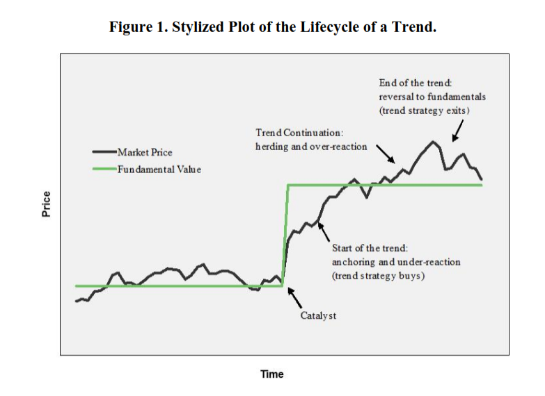
Start of the trend: Under-reaction to information
- Markets may underreact due to:
- anchoring
- disposition effect – people tend to sell winners too early and ride losers too long (Shefrin & Statman (1985), Frazzini (2006))
- non-profit-seeking activities – central banks manipulate currency and fixed-income prices to reduce volatility; some investors mechanically rebalance
- frictions and slow-moving capital
Trend continuation: Delayed overreaction
- Markets may overreact due to:
- herding
- representativeness – people expect assets that went up recently to continue going up
- fund flows and risk management – fund flows often chase recent performance; risk management such as trendfollowing can create feedback loops
End of the trend
- Moskowitz et al. (2012) find evidence that prices mean revert after >1yr, possibly to correct for over-extended trends
Time series momentum across trend-horizons and markets
Identifying and sizing positions
- Go long if an asset has positive excess return (TMOM), and short if negative
- Use 1-month, 3-month, and 12-month TMOM signals
- Positions are sized to target an annualized stdev of 40% for each asset
- Estimate future volatility using exponentially weighted average of past squared returns
- Volatility sizing is important to avoid more volatile assets having a dominant effect on returns
- Rebalanced weekly
- Results are gross of all costs
Performance of the TMOM strategies by individual asset
- Gross Sharpe ratios (CAGR/stdev) for each individual asset under the 12-month rule:
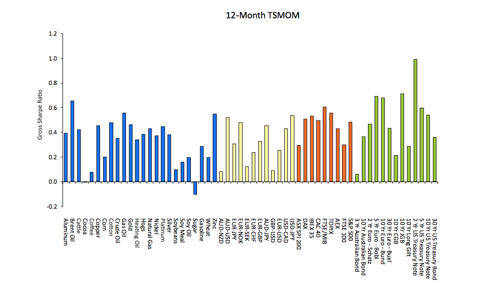
Building diversified TMOM strategies
Historical performance by asset class, 1985-2012
- Constructed by averaging the returns for each trend horizon
- Each basket of assets targets 10% stdev
- alpha is the intercept from a regression on stock + bond + commodity indexes
| Asset | CAGR | stdev | CAGR/stdev | alpha |
|---|---|---|---|---|
| commodities | 11.5 | 11.0 | 1.05 | 12.1 |
| equities | 8.7 | 11.1 | 0.78 | 6.8 |
| fixed income | 11.7 | 11.7 | 1.00 | 9.0 |
| currencies | 10.4 | 11.9 | 0.87 | 10.1 |
| diversified | 19.4 | 10.8 | 1.79 | 17.4 |
Historical performance by time horizon
| Asset | CAGR | stdev | Sharpe | alpha | alpha/stdev |
|---|---|---|---|---|---|
| 1-month | 12.0 | 9.5 | 1.26 | 11.1 | 1.17 |
| 3-month | 14.5 | 10.2 | 1.43 | 13.3 | 1.3 |
| 12-month | 17.2 | 11.3 | 1.52 | 14.4 | 1.27 |
Diversification: Trends with benefits
- Average pairwise correlation across individual assets is close to 0
Asset classes have low correlations:
commodities equities fixed income currencies commodities equities 0.2 fixed income -0.1 0.1 currencies 0.1 0.2 0.1 - me: this suggests that there is no "trend factor", or else the different asset classes would show trends at the same time
Trend horizon correlations:
1-month 3-month 12-month 1-month 3-month 0.6 12-month 0.4 0.6 - Diversified TMOM strategy has low correlations to long-only indexes: r=0 with S&P, r=0.23 with Barclays US Aggregate, r=0.05 with GSCI
- Volatility weighting helps to improve diversification. Example: 5-year US bonds have 5% stdev, while natural gas futures have 50% stdev
- TMOM performs best in strong bull or bear markets, and weakly in flat markets
Time series momentum explains actual managed futures fund returns
- Managed futures indexes, as well as the top 5 biggest managed futures managers, have positive alpha relative to stock + bond + commodity indexes, and most are statistically significant (net of all costs)
- A 2-and-20 fee structure results in about a 6% total fee for the diversified TMOM strategy. Then add 1-4% transaction costs. This reduces TMOM gross Sharpe from 1.79 to ~1.0
- Managers have minimal alpha on a regression of the 1/3/12-month TMOM strategies, or on a regression of the four asset-class TMOM strategies
- A regression on 1-month, 3-month, and 12-month TMOM has an r2 varying from 0.36 to 0.64 for managed futures funds. Correlations to our TMOM strategy range from 0.66 to 0.78
- Most managers have negative alpha on this regression. "This is an illustration of the importance of fees and transaction costs"
Implementation: How to manage managed futures
- Effect of rebalance frequency: MF-rebalance-frequency.png
- Garleanu & Pedersen (2013) derive an optimal portfolio-rebalancing rule to account for transaction costs, which puts more weight on longer-term trend signals
- The TMOM strategy would probably require institutional investors to post ~10% margin, and small investors 20+%
AQR: Can Risk Parity Outperform If Yields Rise? (2013) assetallocation finance
Exeuctive Summary
- Risk parity can outperform in a moderately rising rate environment, even if the cumulative rate increase is large
- Short periods of sharply rising rates can hurt any asset allocation strategy, but risk parity is likely more vulnerable to rate shocks than traditional approaches
- Risk parity offers a modest but real edge over traditional asset allocations, outperforming a little more often than not
- Over the long term, we believe diversification should win
Rising Rates — What, Me Worry?
- Rates dropped from ~4% in 1926 to 1.6% in 1945, rose to 15.8% in 1981, and dropped back to 1.6% by 2013
- We test a strategy that puts equal risk in global equities, bonds, and commodities, targeting 10% standard deviation
- Forecast expected asset volatility by looking at prior 12-month volatility
- Rebalance monthly
- Risk parity using only US stocks and bonds would have underperformed 60/40 in the 1947-1981 period
Historical performance 1947-1979 (moderately rising rates)
| Strategy | CAGR | stdev | Sharpe |
|---|---|---|---|
| 60/40 US | 7.5 | 8.8 | 0.42 |
| 60/40 Global | 8.7 | 6.8 | 0.72 |
| Risk Parity | 11.9 | 10.0 | 0.81 |
Historical performance 1979-1981 (rapidly rising rates)
| Strategy | CAGR | stdev | Sharpe |
|---|---|---|---|
| 60/40 US | 0.0 | 13.0 | -0.98 |
| 60/40 Global | 3.1 | 11.7 | -0.82 |
| Risk Parity | -6.7 | 14.4 | -1.35 |
Historical performance 1981-2013 (falling rates)
| Strategy | CAGR | stdev | Sharpe |
|---|---|---|---|
| 60/40 US | 11.0 | 10.1 | 0.65 |
| 60/40 Global | 10.5 | 9.7 | 0.63 |
| Risk Parity | 12.8 | 9.3 | 0.90 |
Rising Rates — Speed Matters
- How equities respond to unexpected rising rates depends on whether the higher expected cash flows from earnings/dividend growth outweigh the higher discount rate
- Bonds still outperformed cash during the period of rising rates
- The market usually expects rates to rise, which leads to an upward sloping yield curve. If rates do moderately rise, bonds still earn a risk premium
- Equities performed unusually well over the full period (P/E rose from 11 to 23), while bonds did not (starting and ending yields are about the same); but risk parity still outperforms the equity-heavy 60/40 portfolio
Asset class performance during each sub-period
1947-1979
| Asset Class | CAGR | stdev | Sharpe |
|---|---|---|---|
| Stocks | 11.1 | 10.2 | 0.71 |
| Bonds | 4.2 | 3.0 | 0.12 |
| Commodities | 14.6 | 15.4 | 0.70 |
| Cash | 3.8 |
1979-1981
| Asset Class | CAGR | stdev | Sharpe |
|---|---|---|---|
| Stocks | 10.0 | 12.4 | -0.22 |
| Bonds | -1.3 | 11.2 | -1.26 |
| Commodities | -3.0 | 17.5 | -0.90 |
| Cash | 12.7 |
1981-2013
| Asset Class | CAGR | stdev | Sharpe |
|---|---|---|---|
| Stocks | 9.7 | 14.5 | 0.36 |
| Bonds | 9.7 | 6.3 | 0.83 |
| Commodities | 6.3 | 13.4 | 0.14 |
| Cash | 4.4 |
Full
| Asset Class | CAGR | stdev | Sharpe |
|---|---|---|---|
| Stocks | 10.4 | 12.5 | 0.48 |
| Bonds | 6.6 | 5.3 | 0.43 |
| Commodities | 9.9 | 14.5 | 0.39 |
| Cash | 4.3 |
Notes me
- Outperformance of AQR's simulated risk parity strategy 1947-1981 is due to commodities + global diversification, not bonds–the paper even says that risk parity with only US stocks/bonds underperforms. The real takeway isn't risk parity, but diversification beyond US stocks/bonds
- Commodities returned 14.6% 1947-1979 which is kind of crazy
- Commodity futures were in perpetual backwardation back then so performance probably won't repeat itself
- T-bills outperformed 10-year bonds 1947-1981 (4.4% vs. 2.9%, with stdev 3.1% vs. 4.9%) so there was just zero reason (in hindsight) to hold bonds over T-bills (data source)
- And since you pay the T-bill rate (or more) for leverage, de-leveraging is strictly superior to holding T-bills
- AQR claims that bonds outperformed cash 1947-1981, which is inconsistent with my data source
Asness: Risk Parity: Why We Lever finance assetallocation
https://www.aqr.com/Insights/Perspectives/Risk-Parity-Why-We-Fight-Lever
- A risk parity investor can build a higher-return-for-risk-taken portfolio, which more than compensates for the necessity of employing leverage
- Two crucial ingredients of a risk parity strategy:
- Asset allocation must be balanced by risk, not by dollars. Need not be exact parity, but should be biased toward risk balance
- If expected return is too low, apply leverage rather than changing asset allocatio2. If expected return is too low, apply leverage rather than changing asset allocation
- Compared to traditional portfolios, the risk parity portfolio almost always has more weight in bonds and diversifiers (like commodities)
- Low-risk assets tend to have higher risk-adjusted returns than they 'should' have. See Leverage Aversion and Risk Parity. Related to the low-vol anomaly
- Leverage aversion makes people under-invest in low-risk assets
- Excessive leverage is dangerous, but there are things you can do to ameliorate
- Can reduce leverage when market risk looks higher
- Can reduce leverage after losses to avoid seeing bigger losses, and then add back leverage later (which psychologically is the harder part)
- Leverage may appear particularly dangerous right now as bond yields are low; but stocks are expensive as well, so the optimal portfolio still includes bonds
- :me: this is less true if you include emerging markets and value/momentum
- 1947-2014 saw bond yields take a round trip while equity valuations increased, so over this period a portfolio with more equity weighting should have done unusually well; but risk parity still outperformed
- Simulations show that risk parity would have outperformed during long periods of rising rates (from superior diversification and the fact that bonds can still deliver a positive return even when rates rise modestly). Risk parity only performs poorly when rates rise sharply, or when equities outperform in general
Notes me
I think there are three key arguments against risk parity with leverage:
- bond yields are really low
- theoretical models assume leverage costs RF, but it costs me more than RF
- stocks can outperform via value/momentum; bonds cannot
This article touches on point 1 (the below article addresses it further), but it does not address 2 or 3 so I'm still unconvinced.
AQR Risk Parity Fund (AQRIX) holdings as of 2018-09
https://funds.aqr.com/our-funds/global-allocation-funds/risk-parity-fund
| Asset | % |
|---|---|
| stocks | 27 |
| nominal bonds | 23 |
| commodities | 25 |
| inflation-linked bonds | 2 |
| credit | 16 |
| currencies | 7 |
- according to fact sheet, focuses on four risks: equity, nominal interest rate, inflation, and credit/currency
Asness: The Interaction of Value and Momentum Strategies finance value momentum
The Interaction of Value and Momentum.pdf
- Value is strongest among low-momentum stocks and momentum is strongest among expensive stocks
- Cheap stocks still have normal momentum spreads and high-MOM stocks have normal value spreads, which means value has higher explanatory power among low-momentum stocks and vice versa
- Any explanation for why value and momentum work must explain this interaction
Introduction
- Suppose B/M outperforms because it is a proxy for distress. A high-momentum stock is unlikely to be distressed, so B/M is not a symptom of distress in that case
- Suppose B/M outperforms because investors are uncomfortable with buying cheap stocks. If investors are not uncomortable with recent winners then that explains why B/M does not work for momentum stocks
- :me: typical explanation of momentum is that people under-buy high-momentum stocks (aka they're uncomfortable with buying 'too high'), which contradicts this
Sorting on both variables
- B/M for individual stocks is adjusted for industry: "true" BM = log(BM(stock)) - log(BM(industry)), using Fama-French 49 industries
- B/M works better when adjusting for industry average
- Monthly return for bottom and top 20% B/M from within top 20% momentum is 1.50% vs. 1.62% (statistically insignificant)
- But B/M spread among top-momentum stocks is as big as for the market in general, which means B/M is less predictive
- A long/short momentum strategy among the expensive quintile outperforms a long/short over the cheapest quintile (t=3.50)
- Mathematically equivalently, long/short value over losers outperforms long/short value over winners
- :me: Another way to say this is that in a 5x5 grid of value & momentum quintiles, the high/low corners outperform the high/high plus low/low corners
Conclusion
- Dividend yield is a weak value metric in general, but works well among low-momentum stocks (92bps monthly return spread for bottom quintile vs. 32bps spread for market)
Me
- Based on Table 4, the 'VAMO' strategy (buy the 10 buckets closest to the bottom right corner) has 1.44% return, while the 'QVAL+QMOM' strategy (buy Q1-Q5 value and Q1-Q5 momentum) has 1.47%, which is pretty similar
Swedroe: TIPS vs. Nominal Bonds (2018) finance assetallocation
https://www.etf.com/sections/swedroe-tips-vs-nominal-bonds?nopaging=1 (written 2018-08-24)
- As of writing, 5-year treasuries yield 2.76% and TIPS yield 0.77% on top of inflation
- Breakeven inflation rate is 1.99%
- Treasuries have to pay a liquidity premium, plus get a discount due to inflation risk
- Fed survey projects a 10-year inflation of 2.2%; five-year inflation swaps are priced at 2.4%. These suggest TIPS are actually priced at a discount to inflation risk
- Some academic papers (1, 2, 3) argue that investors should strongly prefer TIPS unless the inflation risk premium is large
- Authors of #2 concluded that with no inflation risk premium, optimal TIPS allocation is 80%; with a 0.5% premium, optimal allocation is 60%
- CDs may pay higher rates than treasuries, in which case they might be preferred to TIPS
- Top 5-year CD rates are 3.4%, which implies an inflation risk premium of 0.2%-0.4% (depending on what inflation estimate you use)
- Short-term bonds are a poor inflation hedge because they're too slow to react to unexpected inflation, and frequently pay negative real rates anyway (as they do today)
Azeria Labs: The Importance of Deep Work and the 30-Hour Method for Learning a New Skill self_optimization
https://azeria-labs.com/the-importance-of-deep-work-the-30-hour-method-for-learning-a-new-skill/
- There are lots of available learning resource which makes it hard to start
- When we want to learn something, we usually get struck by motivation, mess around with it for a while, then run out of motivation and give up
- Instead you should start with action, which sparks motivation
- To consistently create a state of flow, you must engage in deep work
- Introduce routines and rituals to minimize the amount of willpower necessary to transition from a distracted state into flow
- Takes ~25 minutes of focus without distraction to get into flow
- Shallow work: Non-cognitively demanding, logistical-style tasks. Do not create much value in the world and are easy to replicate
Putting it into practice
Some possible strategies, extracted from Cal Newport's "Deep Work":
- Monastic: eliminate shallow obligations & distractions
- Bimodal: divide time between deep work and free; dedicate a few consecutive days to pure deep work
- Rhythmic: daily habit of 3-4 hours every day to do deep work
- Journalistic: do deep work wherever it fits into your schedule (harder)
"But I don't know which topic to focus on"
- Pick a skill that can be useful to your current path. Give it a try for a minimum of 30 hours of deep work
- Split your 30 hours into seven 4-hour sessions (plus buffer). Set clear goals
- Use your first session to perform exhaustive information gathering. Pick most useful resources
- If applicable/necessary, use the second session to set up the environment
Example: ARM exploitation
Work sessions
- Information gathering and reading
- Setting up an environment
- Install a VM
- Learn basic commands
- Practice with simple Stack Overflow challenges
- Continue Session 3
- Solve ARM challenges. Get advanced challenges from root-me.org
- Continue solving advanced challenges
- Continue solving advanced challenges
HN Comments
/u/jonathanfoster
Newport's "Deep Work" contains actionable advice such as:
- Create a to-do list each day and separate tasks into shallow and deep categories
- Block off each hour of the day and fill it with one of the to-do items
- Restrict shallow work to 2 hours (after 2 hours, say no to everything shallow)
- Create a scorecard and track the number of deep hours each day
- Experiment with Newport's recommendations for two weeks and see which ones increase your deep hours
- Become comfortable saying no
/u/RobertoG
It seems that the reason flow state is difficult to achieve is because the task has to have the proper difficulty. Too easy and it's boring; too hard and it's frustrating.
Blitz: Are Exchange-Traded Funds Harvesting Factor Premiums? finance factors
https://mdickens.me/materials/org/Blitz-%20ETF%20Factors.pdf
Overall, ETFs do not have significant loading on any factor (size, value, momentum, low-vol) except market beta
SMB HML MOM LV-HV exposure 0.03 -0.03 0.01 0.00 alpha 1.4 -1.3 1.0 -0.3 Smart beta ETFs have statistically significant but weak (<0.1) positive loading on value and low-vol, while non-smart-beta ETFs have weak negative loading. No significant weighting on momentum
SMB HML MOM LV-HV smart-beta exposure 0.25 0.08 0.03 0.06 smart-beta alpha 7.9 2.3 1.3 2.4 conventional exposure -0.06 -0.08 0.01 -0.03 conventional alpha 2.6 3.1 0.6 1.8
Wes Gray: Momentum Investing- Simple, But Not Easy finance momentum
Crowding
- 14min: Blitz, "Are Exchange-Traded Funds Harvesting Factor Premiums?": There are as many ETFs with negative loading on momentum as positive loading, and the most momentum-loaded ETFs aren't even explicitly about momentum, they're sector funds that happen to have high momentum
- "the market is a lot bigger than a few quant geeks trading momentum"
- 15min: Visual Active Share shows that momentum ETFs like MTUM are barely loaded on momentum
- 18min: "I'd say about 95% of funds don't actually do what they say. They're not actually exploiting any factor"
- 19min: Momentum has had 10+ year underperformance in the 1820's, 1860's, 1900's, 1920's, 1940's, and now. Two of those periods were closer to 20 years
- 24min: I'd put a lot of money on that over the next 100 years, [momentum] is going to work
Jerry Neumann: Power Laws in Venture finance statistics
http://reactionwheel.net/2015/06/power-laws-in-venture.html
- Normal distributions are easy to work with, so if outcomes follow a normal or log-normal distribution, it's easy to account for risk
- Earthquakes, city populations, and wars are power-law distributed: \(p(x) = Cx^{-\alpha}\)
Are venture capital returns power-law distributed?
- Some (such as Peter Thiel) assume VC returns are power-law distributed
- Power laws are hard to distinguish from log-normal distributions
- People like fitting things to normal or log-normal distributions because they are well-behaved; venture capital returns are not well-behaved, and are best described by a power law distribution
What could cause returns to be power law distributed?
- A company's value grows exponentially at rate g
- Time to exit is exponentially distributed with expected time i
Therefore, probability of an exit value of x is:
\begin{align} \frac{1}{gi}x^{-(\frac{1}{gi}+1)} \end{align}- This is a power law distribution with \(\alpha = 1/(gi) + 1\)
- Ignores some important details, e.g. growth rates tend to slow over time. But it basically explains the power-law-ish distribution of VC returns
- :me: this model can have infinite EV, but only with infinite time, because the way it has infinite EV is that companies can continue growing exponentially for arbitrarily long
Venture capital power law distributions
- VC firms hold investments for an average of 4 years and expect 26% CAGR which gives parameter value \(\alpha = 1.96\)
- :me: in podcast he said alpha was slightly below 1, but the alpha parameter is used in two different ways so this is consistent
- Other sources estimate alphas 1.68 to 2.27, with a median of 1.85
- Later-stage ventures have larger alpha
Some alphas for non-VC innovative activity
| value of patents | 1.3-1.7 |
| size of all US firms | 2.1 |
| corporate R&D | 2.2 |
| size of S&P500 firms | 2.3 |
| movie income | 2.9 |
Infinite mean
- If \(\alpha < 2\), mean is \(\infty\)
- When \(\alpha = 2\), with a sample of size n, the mean of the largest sample value is n. If you invest in 10 companies, the likeliest largest return is 10x
- When \(\alpha < 2\), mean value of largest pick is greater than n
Alphas close to 2
- Why do VC alphas cluster so close to 2? Why not go even lower?
- One reason is timing: a 10 year fund wants most of their investments to exit within 10 years, so they need to target ~5 year mean time to exit
- Getting lower alpha is constrained by finding enough companies who can generate sufficient growth in the required time period
- Best explanation is supply and demand: VCs eat up all the investments with \(\alpha < 2\)
Unresolved questions
Failure rates
- Better fund returns (i.e. fatter tail) coincide with more faiures (i.e. fatter head). But a power law distribution cannot have both a fatter head and a fatter tail b/c the area must sum to one
SSC: Melatonin: Much More Than You Wanted to Know health
- To fall asleep and wake up earlier, take melatonin 5 hours prior to bodily melatonin production, which is probably about 7 hours before going to sleep
- To fall asleep and wake up later, in theory you could take melatonin first thing in the morning. This has never been studied, but researchers say it should work
Gray & Vogel: Analyzing Valuation Measures (2012) finance value
Analyzing Valuation Measures: A Performance Horse-Race over the Past 40 Years
- Contra Fama & French, there are economically and statistically significant differences in the performance of various valuation metrics
- Under consideraton: E/P, EBITDA/EV, FCF/EV, GP/EV (gross profit), B/M, forward E/P
- 1971 to 2010, EBITDA/EV (top quintile) performs best: 17.7% annualized return with 2.91% 3-factor alpha
- E/P, the most popular metric, has no significant 3-factor alpha
- forward E/P is by far the worst metric
- EBITDA/EV has 9.7% spread between cheap and expensive quintiles return
- E/P has only 5.8% spread
- Long-term valuation metrics (e.g. CAPE) provide no improvement
Data
- Excludes REITs ADRs, closed-end funds, utilities, financials
- Incorporates CRSP delisting return data using Beaver, McNichols, and Price (2007)
- Restrict to firms with 8 years of data so we can make apples-to-apples comparison with long-term metrics
- For liquidity, restrict market cap to >10th percentile NYSE breakpoint
- EV = M + DLC + DLTT + PSTKRV + CHE
- Book value is CEQ + PSTK or AT - LT
- Can measure preferred stock with either PSTKRV or PSTK
A Comparison of valuation metrics
Valuation metric performance
- Mkt = equal-weighted market
- alpha is for top quintile
| Top | Top-Bot | alpha | t-stat | |
|---|---|---|---|---|
| E/P | 16.0 | 5.5 | 1.3 | 1.4 |
| EBITDA/EV | 17.7 | 9.7 | 2.9 | 3.3 |
| FCF/EV | 16.6 | 5.5 | 2.9 | 3.9 |
| GP/EV | 16.5 | 8.2 | 2.1 | 2.3 |
| B/M | 15.0 | 5.8 | -0.7 | -0.7 |
| Mkt | 13.0 | N/A | N/A | N/A |
- FCF/EV has most significant predictive power for the top quintile, but weak on the bottom quintile
- EBITDA/EV has highest top quintile return and biggest top-bottom spread
- E/P (and B/M obvs) do not have significant alpha; others do
- Results look comparable on the 1991-2010 period (aka after Fama&French publication)
Valuation metric risk
- Sharpe and Sortino ratios are based on monthly returns
| Sharpe | Sortino | MaxDD | |
|---|---|---|---|
| E/P | 0.17 | 0.23 | -51 |
| EBITDA/EV | 0.19 | 0.26 | -55 |
| FCF/EV | 0.18 | 0.25 | -52 |
| GP/EV | 0.17 | 0.24 | -63 |
| B/M | 0.15 | 0.20 | -61 |
| Mkt | 0.13 | 0.19 | -56 |
- EBITDA/EV and FCF/EV have best Sharpe and Sortino ratios
- For value-weighted portfolios (not reproduced here), all drawdowns are lower, with EBITDA/EV and FCF/EV being the lowest at -43% and -42%
- We compared these metrics against forward E/P based on earnings estimates, and forward E/P was easily the worst
Examining long-term valuation measures
Long-term valuation metric performance
- Little evidence that normalizing the numerator (EBIT, FFC, etc.) predicts higher portfolio returns
- Anderson and Brooks (2006) found that long-term metrics work better in the UK stock market but we were unable to replicate in the US
Value
| Metric | 1yr | 3yr | 8yr |
|---|---|---|---|
| E/P | 16.0 | 16.1 | 15.8 |
| EBITDA/EV | 17.7 | 17.4 | 16.5 |
| FCF/EV | 16.6 | 15.9 | 15.1 |
| GP/EV | 16.5 | 16.7 | 16.6 |
| B/M | 15.0 | 15.5 | 15.6 |
Spread (Value - Growth)
| Metric | 1yr | 3yr | 8yr |
|---|---|---|---|
| E/P | 5.5 | 5.9 | 6.1 |
| EBITDA/EV | 9.7 | 10.0 | 9.3 |
| FCF/EV | 5.5 | 4.7 | 3.2 |
| GP/EV | 8.2 | 8.6 | 8.3 |
| B/M | 5.8 | 7.5 | 7.5 |
Robustness of valuation metrics across the business cycle
- Which metric performs best could depend on economic regime. Perhaps FCF will work better in economic downturns, and B/M will work better when economy is manufacturing-focused and less well when it's human capital-focused
- We analyze valuation metric performance during economic expansions and contractions as defined by the National Bureau of Economc Research
- No clear evidence that a particular metric outperforms during contractions
- Ex. GP/EV had the strongest return (29%) in the 1981-1982 contraction, but the worst performance (-22%) during 2007-2009
- Value metrics do outperform on average during both expansions and contractions
Conclusion
- EBITDA/EV has historically performed best, based on looking at absolute performance, risk metrics, and 3-factor alpha
- Long-term ratios add minimal value
- No particular value metric performs best during expansions or contractions, but value as a whole outperforms in good times and bad
Corey Hoffstein: Factor Fimbulwinter finance factors
https://blog.thinknewfound.com/2018/06/factor-fimbulwinter/
- If value (aka long-short B/M, aka HML) no longer works, it will take in expectation 67 years before the value premium is no longer statistically significant at p=0.01
Swedroe: Role of REITs in a Diversified Portfolio finance alternatives
http://thebamalliance.com/blog/the-role-of-reits-in-a-diversified-portfolio/ local PDF
REITs have historically low correlation with stocks and bonds (r=0.6 with stocks), and returns are not well-explained by the single-factor CAPM. But does that mean REITs are a useful diversifier?
Kizer & Grover (2016), "Are REITs a Distinct Asset Class?"
An asset class qualifies as distinct if it meets these criteria:
- Low correlation with established asset classes
- Statistically significant positive alpha with respect to factor models
- Inability to be replicated by a long-only portfolio holding established asset classes
- Improved mean-variance frontier when added to a portfolio holding established asset classes
Do REITs produce factor model alpha?
- Use a six-factor model with four equity factors (market, size, value, momentum) and two fixed income factors (term and credit)
- credit = corporate bonds - Treasuries
- Study examined REITs plus 12 industries on Ken French's website (presumably 12 Industry Portfolios)
- Six-factor model explains nearly all industries' returns; only exception was the "other" industry (Mines, Constr, BldMt, Trans, Hotels, Bus Serv, Entertainment), which had negative alpha
- REIT alpha had t-stat -0.3, aka highly insignificant
- REITs showed statistically significant exposures to market beta, size, value, term, credit
Can REITs be replicated by a portfolio of established asset classes?
- Attempt to replicate with small-cap value + corporate bonds (67%/33% weighting)
- r=0.72 with REITs
Summary stats (this portfolio beats REITs in every way)
REITs Portfolio CAGR 12.5 14.3 stdev 19 14 Sharpe 0.49 0.73 MaxDD -71 -47 - Interest rates declined during tested period (1978-2016) which could explain some of Portfolio's performance, but REITs have a higher loading on term factor than Portfolio so that doesn't explain it
Stelk, Zhou & Anderson (2017), "REITs in a Mixed-Asset Portfolio: An Investigation of Extreme Risks"
Insights from literature review(ception)
- Unexpected monetary shocks affect REITs about twice as greatly as they affect the general equities market under high-variance regimes
- In int'l markets, REITs are more likely to see extreme price swings, and they tend to coincide with broad market swings
- REITs are riskier than the broad market in each of seven countries studied
- Stock and REIT returns are significantly more correlated during downturns
- Of several alternative asset classes studied, REITs had the highest correlation to stocks and bonds (https://www.cfapubs.org/doi/full/10.2469/dig.v42.n4.10)
- from abstract: commodities provide best diversification, and within commodities, gold is best diversifier and industrial metals are worst
Findings
- Adding REITs to a mixed-asset portfolio does not have significant impact on the average daily return or value at risk of a portfolio prior to 2006 (aka prior to GFC)
- After 2006, adding REITs significantly increases value at risk
Van Nieuwerburgh (2017), "Why Are REITs Currently So Expensive?"
- Examined Vanguard REIT Index Investor Fund (VGSIX)
- 1996-2007, VGSIX had factor loadings beta: 0.53, size: 0.38, value: 0.75, momentum: -0.05 (r=0.60)
- 2008-2017, VGSIX had factor loadings beta: 1.02, size: 0.13, value: 0.46, momentum: -0.15 (r=0.77)
- REITs have market beta 1.75 2006-2010, which was the worst period to have high market beta
- REITs didn't used to have much interest rate risk but now they have a lot, which is bad considering how low rates are (if rates go up, REITs will suffer)
Conclusion
- REITs should not be excluded, but they should only receive market-cap weighting at most
- At Buckingham, the equity mutual funds we use exclude REITs, so we add a separate allocation of about 3% to REITs
- Investors concerned with downside risk should consider reduced allocations to REITs (below 3%)
Stock options and the Alternative Minimum Tax finance taxes
- If you pay AMT, the amount it exceeds your regular tax gets carried forward as a credit. Then in a future year if your regular tax exceeds AMT, you can apply the credit against the difference
Serge Fauget: Biohacking self_optimization health
Sleep hygiene
- Bedroom should be very dark, and cold (18-19C)
- Wake up at the same time every morning
- Reduce activities that disrupt sleep (e.g. alcohol, evening exercise)
- Sleep is essential to willpower, which is essential to everything else here
Optimal nutrition
- Do not eat sugar (candy, fruit juice, bread, pasta, honey, etc.)
- Eat organic
- Don't drink alcohol (screws up sleep) and don't add salt to food (increases blood pressure)
- I do intermittent fasting where for 3 days a week I only eat once a day
Optimal exercise
- Lift weights 2-3x/week, focusing on hip-hinge exercises to build maximum muscle (squats, deadlifts)
- HIIT 2-3x/week
- I do 5 min warmup, 8 sets of 20-30 sec fast + 60-90 sec slow, 5 min warmdown
- Standing desk
Mental health
- Meditations
- See Waking Up by Sam Harris
- Psychotherapy
- I discuss questions like "How do I eliminate bad mood days?", "How do I find it trivially easy to always chat with girls I find attractive?"
- Never lie
Supplements & drugs
- Metformin (1g morning + 1g evening): anti-diabetes drug that lowers blood sugar. Beneficial in preventing cancer and heart disease; currently in FDA trials as anti-aging treatment
- Lithium carbonate (150mg/day): mood stabilizer, possibly beneficial cognitive effects. Negative effects in higher doses so don't have more
- Modafinil (200mg/day)
- SSRI escitalopram (10mg/day): makes everything a little bit nicer and more enjoyable
- MDMA one time: got rid of social anxieties and made me more extroverted and sexually liberated
Supplements that are quite likely to be useful
- bacopa monieri
- creatine
- olive leaf extract
- trimethylglycine
- magnesium threonate
- R-lipoic acid
- curcumin
- vitamin K2 MK4/7
- ashwagandha
- garlic
- omega-3
- B12
- coenzymate-B complex
- vitamin D
- CoQ10
AlphaArchitect: A Tactical Asset Allocation Horserace Between Two Thoroughbreds finance trend assetallocation
Strategies
Dual Momentum
- Apply dual momentum to four pairs of assets; pick whichever asset has higher relative momentum; if both have negative absolute momentum, go to cash
- Asset pairs
- equity: US equity, int'l equity
- real estate: equity REIT, mortgage REIT
- stress: gold, long-term bonds
- credit: high yield bonds, BBB rated bonds
Robust Asset Allocation
- Asset classes are the same as dual momentum: US equity, int'l equity, equity REIT, mortgage REIT, gold, long-term bonds, high-yield bonds, BBB rated bonds
- Invest 100%/50%/0% based on time-series momentum and simple moving average trendfollowing rules
RAA and Dual MOM Horserace by Asset Pair
- Gross returns (no fees or transaction costs), rebalanced monthly
- Consider one strategy a winner if it has better Sharpe and Sortino ratio; if neither wins on both, it's a tie
- Compared on each asset (pair):
- equity: Dual MOM
- real estate: RAA
- stress: RAA
- credit: RAA
- 8 asset mix (equal-weighted): RAA
- 6 asset mix (excl. credit): RAA
- out-of-sample 6 asset mix: Tie
- Dual MOM had better CAGR in every case, and RAA had better stdev + downside dev in every case
- me: Sharpe/Sortino ratios are pretty similar overall
Nader Al-Naji: A Rigorous Framework for Evaluating Startup Compensation finance career
- You should prefer $4 of equity over 4 years to $1 of salary, because if the company does well, the equity will be worth >$1 per year, and if it does poorly, you can just go work somewhere else
- You may have to pay AMT on the difference between the FMV and the strike price, but when you sell, you can get a tax credit that effectively means you only paid cap gains tax (if you have ISOs)
- To avoid concerns with illiquidity, avoid companies issuing high-strike-price options unless they're about to IPO; and early exercise to avoid AMT
- Getting paid in ISOs is more tax-efficient than cash because you'll pay capital gains tax instead of income tax (if you avoid AMT)
Covel: The Complete TurtleTrader finance books trend
Strategy (chapter 5)
System 1. Buy if price exceeds 4 week high. Exit if price drops below 2 week low. Only buy if previous buy signal was not a winner.
System 2. Buy on 11 week high, exit on 4 week low.
Put half your money into each system.
Always exit on 2N stop: if price drops 2 standard deviations below the 4 week daily average.
Try it on http://wealthlab.com/.
AQR: Hedge Funds – The (Somewhat Tepid) Defense finance alternatives
https://www.aqr.com/cliffs-perspective/hedge-funds-the-somewhat-tepid-defense
- Hedge funds are generally too expensive and don't hedge well enough
- That said, it's not fair to pick on hedge funds for underperforming the S&P because they're supposed to have beta < 1
- Caveat: hedge fund index data is potentially biased for several reasons including survivorship bias
- Hedge fund return % predicted by `y = 3.5 + 0.37x`, where `x` = S&P return
- `r2 = 0.57`
Hedge funds vs. 60/40, 1994-2014
| Stocks | 60/40 | Hedge Funds | |
|---|---|---|---|
| Compound Return | 9.3 | 8.3 | 8.7 |
| GFC Return | -49 | -30 | -17 |
| Max Drawdown | -51 | -33 | -21 |
MVO
- MVO over [stocks, bonds, hedge funds], targeting the same volatility as 60/40, outputs [31% stocks, 0% bonds, 69% hedge funds]
- 9.1% annualized return
MVO with leverage
- New MVO result is [0% stocks, 227% bonds (lol), 90% hedge funds]
- 15.3% annualized return
- Hedge funds are sufficiently correlated with equities that MVO prefers to leave out stocks
AlphaArchitect: Berkin and Swedroe's Factor Investing Book finance factors
Our ratings of factors
(roughly in order of evidence and sustainability out of sample)
AlphaArchitect: How to Pick Smart Beta ETFs finance factors
http://blog.alphaarchitect.com/2015/10/24/how-to-pick-smart-beta-etfs/
- "Closet indexes" are more expensive than they look because you're paying a lot for exposure
- Consider not the expense ratio of the fund, but how much you're paying relative to how much exposure you're getting
Closet value index vs. replication value
- Funds
- Concentrated Value: top 5% of value stocks, equal-weighted
- Diluted Value (closet index): top 33% of value stocks (by B/M), value-weighted
- Replication Value: 70% invested in the market, 30% invested in Concentrated Value
| Strategy | CAGR | Sharpe | Sortino |
|---|---|---|---|
| Concentrated | 14.3 | 0.53 | 0.76 |
| Diluted | 11.3 | 0.45 | 0.63 |
| Replication | 11.4 | 0.45 | 0.63 |
- Diluted Value and Replication Value perform almost exactly the same
- If Replication Value costs 0.7% more than the market, we can pay 0.21% extra for the same value exposure as Diluted Value
- That makes Vanguard value ETF cheaper than Replication Value, DFA about the same, and AQR more expensive
The Real-Estate Crowdfunding Review: Why not a REIT? finance alternatives
http://www.mrmoneymustache.com/2016/05/02/peerstreet/
- From 1978 to 2014, REITs experienced much more volatility than a direct real estate index
- REITs lost money 8 years and direct real estate only lost money 4 years
- REITs lose money whenever the stock market does, so worse diversification than direct real estate
- "Departures from NAV in REIT Pricing" found that REIT owners pay extra costs for getting liquidity
Meb Faber: A Quantitative Approach to Tactical Asset Allocation (2006) finance trend
Market timing
- Buy when price > 10-month simple moving average (SMA), move to cash when price < 10-month SMA
S&P 500 returns with and without timing, 1900-2005:
S&P timing CAGR 9.8 10.7 stdev 19.9 15.4 Sharpe 0.29 0.43 drawdown 84 50 - SMA is robust: performs well for different periods (6, 8, 10, 12, or 14 months) and for different asset classes (S&P, EAFE, bonds, GSCI, REIT)
Asset allocation
Returns equal-weighted across US stock (S&P 500), int'l stock (EAFE), 10-year bonds, commodities (GSCI), and real estate (NAREIT) from 1972-2005:
AA timing timing 2X S&P CAGR 11.6 11.9 16.6 11.2 stdev 10.0 6.6 13.9 17.5 Sharpe 0.75 1.20 0.90 0.41 drawdown 20 10 21.9 45 - 2x leverage stats include borrowing costs
Practical considerations
- Timing does not affect management fees and only slightly increases commissions because you only make 3-4 round trip trades per year (less than one per asset class)
- Large tax hit if trading in a taxable account
- But this system does tend to produce short-term losses and long-term gains
Gray & Kern: ValueInvestorsClub Performance (2008) finance value
title is "Fundamental Value Investors: Characteristics and Performance" (2008) https://mpra.ub.uni-muenchen.de/12620/1/MPRA_paper_12620.pdf or file:///home/mdickens/Documents/Reading/ValueInvestorsClub.pdf
- Value Investors Club primarily includes hedge fund managers and activist investors so it represents a good selection of successful value investors
Characteristics of decisions
- Participants overwhelmingly focus on assessing intrinsic value
- 98% of recommendations cite three or fewer investment criteria
- Median Price/Book of recommendations is 1.6, which is slightly higher than market P/B
Performance
- 33% annualized return
- 19% return over the market
- One-year performance over period 2000 to 2008
(note: according to AlphaArchitect blog, Value Investors Club performed worse than QVAL over the sample period)
The Joel Test programming
- Do you use source control?
- Can you make a build in one step?
- Do you have daily builds?
- Do you have a bug database?
- Do you fix bugs before writing new code?
- Do you have an up-to-date schedule?
- Do you have a spec?
- Do programmers have quiet working conditions?
- Do you use the best tools money can buy?
- Do you have testers?
- Do new candidates write code during their interview?
- Do you do hallway usability testing?
- You should score 11 or 12. 10 or lower and you've got serious problems.
Dan Luu: We only hire the trendiest career
http://danluu.com/programmer-moneyball/
- Some companies hire developers based on things like university and previous tech stacks (i.e. not .NET) that don't really matter.
- Moneyball was widely publicized but it took baseball teams years to catch on. Thomas Ptacek @ Matasano and top Google people have been talking for years about how they hire but people still don't listen.
- Companies should put more effort into training and mentorship.
- Good tooling can improve productivity by orders of magnitude; see The Joel Test.
- "I've literally never found an environment where you can't massively improve productivity with something [as trivial as typing up meeting notes]."
Roadmap for Pitching a Venture Capital Firm startups
Podcast from Kleiner Perkins
- Most interesting part of pitch is the "why". Why is this important? Why is it meaningful for you? Why now?
- Show me that there are people who want this
- Numbers in business models aren't worth much because you can't predict where you will be
- But business models are important because I want to see your thinking and how much you've considered your plan
- Most founders don't get to a demo fast enough
- We only fund a company if at least one of our partners loves the idea and is willing to sponsor it
Dunning-Kruger and Other Memes
http://danluu.com/dunning-kruger/
- Dunning-Kruger: People disproportionately perceive themselves as third quartile; perception of ability is correlated with actual ability
- Happiness continues to rise with income even for wealthy people, but the relationship is logarithmic so it's hard to perceive
- Disability, divorce, and unemployent all have long-term negative effects on happiness; lottery winners are happier
Radiolab's "The Bad Show"
- In Milgram's experiment, teachers didn't continue shocking the learners because of obedience to authority. In fact, when experimenters told teachers that they "have no choice," one hundred percent of teachers resisted. Rather, they were motivated by the thought that they have to shock the learner for the greater good of the experiment.
Cracking the Coding Interview career books
Five Algorithm Approaches
- Examplify
- Pattern Matching
- Look for related problems that you know how to solve
- Simplify and Generalize
- Base Case and Build
- Data Structure Brainstorm
- test
Charlie Rose: Levitt and Dubner
- People cause themselves a lot of trouble by caring about things that don't matter
Me
- How to not care about things that don't matter?
- Free kick problem: people don't take risks to avoid looking stupid. But this is probably reasonable, so really we should set up incentives so people are okay with not looking stupid. How?
Ben Hoffman: Werewolf Feelings self_optimization
http://benjaminrosshoffman.com/werewolf-feelings/
- If you tell your friends about a problem they may feel obligated to help you or feel guilty for not helping you
- Low-level werewolves share their problems and high-level werewolves are reluctant to
Whittlestone: Is it ever worth not knowing the truth?
http://aeon.co/magazine/philosophy/is-it-ever-worth-not-knowing-the-truth/
- Some truths are painful at first but eventually helpful (like knowing your boss doesn't like the reports you've been handing in) but some are painful and unhelpful (finding out you have a terminal illness)
- It doesn't benefit me to know that people are suffering in the developing world, but it may benefit them
- The experience machine illustrates that some people intrinsically value truth
- We will either seek too many harmful truths or seek too few useful truths. The latter has a much bigger downside
- I struggle to think of a single time in my life I’ve learned something and seriously wished I’d remained ignorant
- As a rule of thumb, aim to always seek the truth
Steering towards forbidden conversations self_optimization
http://mindingourway.com/steering-towards-forbidden-conversations/
- Difficult conversations are not just less bad than you expect, but actively good
- Teach yourself to subconsciously steer toward difficult conversations
- Adrenaline before a conversation can feel good
- In a story, the difficult conversation is where the plot progresses
Ben Todd on talent gaps career causepri
EAs overlook causes that are talent constrained but not funding constrained
- Examples: foreign policy, climate policy, impactful for-profit orgs (e.g. Wave), scientific research, improving organizational competence
EA favorite causes are talent-constrained
- International development: Charities GW Would Like to See
- EA outreach and prioritization research
- AI safety research: FHI, FLI, CSER have a lot of funding but struggle to find good researchers
- Immigration: few orgs exist that can be funded, so setting one up would be valuable
- Biomedical research: surveyed professors believe an especially good researcher is worth >$100K
- Factory farming does seem more funding-constrained
Balance is likely to shift toward talent constraints in the near future
- Lots of new E2G-ers
- Open Phil ramping up donations
- EA fundraising charities (GWWC, REG, CS) growing
- Direct work not growing as rapidly
Balance is likely to remain in favor of talent constraints in the long run
- EA orgs have a track record of attracting large donors (from Good Ventures, Peter Thiel, Elon Musk)
- EA attracts people with high earning potential
- :me: People with high earning potential heavily overlap with people talented at direct work
- Money is fungible, so it's easier to move money toward funding gaps. Building talented teams takes a long time.
In favor of focusing on funding gaps
- Filling talent gaps requires specialized talents, but anyone can fill funding gaps
- EA is developed enough that it's time to start focusing on talent gaps
What should the community do differently?
- Less earning to give
- Peter Hurford argued that AMF needs money more than people. But GW selected AMF precisely because it's funding constrained.
- Less marginal investment in fundraising projects
- GWWC, TLYCS, ACE, REG, CS. Less effort going into filling talent gaps.
- :me: I don't even know what an organizatian filling talent gaps would look like, except maybe 80K.
- More people exploring new causes
- A community with lots of people in different fields is probably more valuable than one concentrated in a few fields (software, finance)
- Consider doing a PhD, working at a think tank, working in civil service in policy-focused roles, working on emerging-markets tech startups
- More people developing skills for direct work at EA orgs
- People with knowledge of the policy world
- Managers
- Researchers, especially generalists
- Marketing/PR people
- Entrepreneurs/people with experience scaling organizations
- More people doing direct work on top causes
- Better mechanisms for coordinating and solving talent gaps
Greaves: Population Axiology causepri philosophy
Population ethics and population axiology: The basic questions
- Axiology: the ordering over world states
- Even assuming utilitarianism over fixed populations, it is unclear what to do when population size is variable
Totalism and averagism
- Totalism: compare on total well-being
- Averagism: compare on average well-being
- For world state \(X\), let \(|X|\) be the number of people in \(X\), and let \(\bar{X}\) be the average well-being
- \(V_{Tot}(X) = |X| \bar{X}\)
- \(V_{Avg}(X) = \bar{X}\)
- Repugnant Conclusion: Under totalism, for any world A, there is a better world Z where no one has a life more than barely worth living
- Sadistic Conclusion: Under averagism, from a highly positive starting point, it is better to add a small number of people with negative well-being than a large number of people with moderately positive well-being
- Mere Addition Principle: Let A be a world state. Let B be an identical world state but with some extra people with lives worth living. Then B is not worse than A.
- Averagism violates the Mere Addition Principle
Variable Value theories
- Variable Value theory: \(V_{VV}(X) = \bar{X} \cdot g(|X|)\) for increasing and concave function \(g\) with a horizontal asymptote
- This approximates Totalism at small populations and Averagism at large populations
- me: Something like this seems implied by Kevin Gibbons' metaphysical position that repeating an identical state of consciousness provides no marginal value, and adding similar states provides less value than adding novel states.
- Variable Value theories avoid the Repugnant Conclusion because the value of a world asymptotes with the number of people
- It is possible to construct a Variable Value theory that avoids the Repugnant and Sadistic Conclusions while accepting the Mere Addition Principle. But it violates Non-Anti-Egalitarianism
- Non-Anti-Egalitarianism: If worlds A and B contain the same number of people, everyone in B has equal well-being, and B has a higher total well-being than A, then B is better than A
Critical Level theories
- Unlike Average or Variable Value, Critical Level theories accept that the marginal value of a person does not depend on the number or welfare of pre-existing people. But the marginal value of a person equals that person's well-being minus some constant
- Critical Level theory: \(V_{CL}(X) = |X| (\bar{X} - \alpha)\)
- Weak Repugnant Conclusion: For any world A, there is a better world Z where no one has a life more than barely above the critical level
- Critical Level theories violate the Mere Addition Principle and entail the Sadistic Conclusion
Person-affecting views
Neutrality
- Neutrality Principle: Adding an extra person to the world does not make the world better or worse
The principle of equal existence
- Principle of Equal Existence: If worlds A and B are identical except that B has an extra person (with any welfare level), then A and B are equally good
- This is all but self-contradictory: if B1 has an extra person at welfare level 5 and B2 has an extra persona at welfare level 10, then A = B1, A = B2, but B2 > B1
Non-impartial theories
- Forms of non-impartial theories
- Presentism: Only people who presently exist matter
- Actualism: Only actual persons matter (not possible persons)
- Necessitarianism: Persons only matter if they necessarily exist, regardless of the decision
Harm-minimization theories
- The comparative harm to a person in a world state is the amount by which their well-being falls short of the maximum it could have been
- Someone who would not exist otherwise suffers no comparative harm
- The best world is the one with the lowest total comparative harm
- Harm minimization theory violates Independence of Irrelevant Alternatives: bringing someone into existence at welfare level 5 is as good as not, unless you can bring them into existence with welfare level 10, in which case bringing them at 5 is worse than non-existence
Theories with widespread incomparability
- Perhaps world state orderings only hold over fixed populations
- This is intuitively implausible: surely a future paradise is better than a future hell
Impossibility theorems
- There is no axiology that satisfies a set of intuitive requirements
- Attempts at avoiding impossibility theorems:
- The Repugnant Conclusion is, upon deeper inspection, not repugnant (e.g., Tannsjo (2002), Why we ought to accept the Repugnant Conclusion)
- Don't accept that a complete betterness relation exists
- The normative force of impossibility theorems depends on choice-set-independence
- Some claim that impossibility theorems are problematic only for consequentialists. But all moral theories need an axiology
- Even without an axiology, deontological systems face similar impossibility theorems
me
On population axiology and theory of identity:
- Surely, the world where a person lives 100 years is better than the one where they live 50 years, all else equal.
- What if the person goes through a transporter at age 50?
- What if they're cloned at age 50 and the clone lives for another 50 years?
- I haven't quite worked out the right framing of this, but there's something here
Should Open Phil be recommending larger grants? causepri
- Currently prioritizing capacity-building
Case for focusing on grantmaking
- Plans to give hundreds of millions $ per year, currently giving ~$25M so a lot of room to ramp up
- Open Phil hopes to influence other major donors, so may direct a lot more money
- If Good Ventures gives more now, it could help Open Phil attract more funding later
- Haste consideration
- We could recommend more by lowering our standards of diligence
Case for focusing on capacity building
- Currently working on choosing focus areas, hiring people to lead these areas, and working with new hires on their proposed grants
- Program staffers can find better grantmaking opportunities than generalists
- Chloe Cockburn believes she can identify tens of millions of $ of strong opportunities in criminal justice reform
- Have to be careful about hiring program staffers because they need to be value-aligned
- Grantmaking so far was aimed an helping our learning and capacity building
- We will be able to dramatically increase spending soon, so capacity-building only costs a few years
- Other large foundations give away >$100M/year and still consider themselves funding constrained, so we shouldn't expect funding gaps to close in the near future
Could we do both?
We could focus on capacity-building, but make more/bigger grants by doing less due diligence
- Making quicker grants is a new type of activity that would raise unexpected issues
- Grantees want to know the odds of renewal, which takes a lot of work for us to decide
- Our comparative advantage is in careful reflection and not in gut instincts
The plan from here
- By early 2016, we will have been working with program staff for a while and can give them more autonomy
- Should give much more in the next 1-2 years
Good Ventures and Giving Now vs. Later causepri
The basic criteria
Budget
- At peak capacity, will recommend lots of grants
- While learning/building capacity, makes sense to grant 5% per year
Benchmarking against direct cash transfers
- Any grant should look better than cash transfers b/c cash transfers have very large room for more funding
- This standard may be too lax, but right now it isn't obvious how we will find several billion dollars' worth of such opportunities, so we prefer to make more grants
When these criteria apply
- We compare against cash transfers after we've completed an investigation
- We don't investigate every grant that might fit these criteria, just the ones that look best
Complications and adjustments
Exit grants
- Even if we decide to stop funding an org, we may need to give "exit grants" to help the org plan and adjust
- Need to account for this when planning our budget
Knowledge/capacity building
- We're less strict about applying cash transfer benchmark for exploratory grants
Coordination issues
- We don't want to fill the funding gap for every strong opportunity because this creates bad incentives in the long run
"Funging" approaches
- Could give enough to fill whatever funding gaps remain after December giving season
- Incentivizes people not to give to GW top charities
"Matching" approaches
- Could match other donors
- Has opposite incentives from funging: incentivizes donors to give more
- Could produce worse results because total money donated is determined by how much other donors give
"Splitting" approaches
- Could fill our "fair share" of the funding gap
- Provides neutal incentives to other donors
- Donated amount is suboptimal, but better than "matching"
- Can fill most important funding gaps first
Our preference at the moment
- For this year we are using a "split" approach
Specifics of our recommendation re: GiveWell's top charities
- GV will fund 100% of highest-value giving opportunities
- GV will fund 50% of remaining high-value opportunities; not sure how to engineer this choice so 50% is a safe number
Why Open Phil isn't currently funding EA movement-building causepri
Summary
- We give in focus areas rather than one-off opportunities; not worth making EA orgs a focus area
- Having EA orgs as a focus area would require a lot of staff time
- It's not our comparative advantage
- We have discussed ways of funding EA orgs that woudl be less staff-intensive, and may do this in the future
Avoiding one-off grants
- We choose focus areas and ensure that at least one staffer is highly engaged in the area and set clear priorities
- One-off grants take similar work but for much less benefit
- We have strong connections to EAs which makes one-off grants easier, but there are downsides
- Grants/non-grants could be interpreted as endorsement/disapproval, more than is warranted for one-off grants; EAs pay more attention to us than most orgs
- EA orgs might optimize for getting our funding instead of optimizing for transparency and impact. This risk is magnified if we make grants with less serious consideration
EA org grants would be a relatively intensive focus area
- Unlike some focus areas (e.g. land use reform), the field is thick enough that it would require a lot of staff time to keep up
- Conflicts of interest: we are incentivized to help EA orgs that promote GW
- Have to carefully manage relationships with EAs
- There's a risk of amplifying some EA messages that we consider harmful
- EA as obligation
- Overconfident messages ("EA is last social movement we ever need", "global poverty is a rounding error")
Our comparative advantage
Other donors are well-positioned to fund EA orgs
- Most of Open Phil's uniqueness comes from cause selection; within a cause, we work similarly to other orgs
- We don't want to cause others to give less to EA orgs
We are uniquely positioned to apply EA value to outside areas
- We generally avoid "meta" causes because we can do better at meta later if we get a strong sense of the object space in the near term
GiveWell: Importance of committing to causes causepri
http://blog.givewell.org/2014/05/14/the-importance-of-committing-to-causes/
- We're able to find better giving opportunities if we show more interest in a cause
- Many people only make referrals, propose relevant ideas, etc. if they believe you're serious
Approaches we've taken to finding giving opportunities
- Didn't achieve much by asking people which causes to fund, they said the question was too broad
- We found few "shovel-ready" giving opportunities; didn't see how more funding would play a crucial role for existing orgs
- When we looked into meta-research, grant proposals were brought straight to funders who were already known for supporting such research
Examples of the "giving to learn" dynamic
- When we became known for making grants in criinal justice, groups approached us with confidential proposals
The approach we're taking
- Our grantmaking work helps us identify the best causes
Thoughts on the Singularity Institute causepri xrisk
http://lesswrong.com/lw/cbs/thoughts_on_the_singularity_institute_si/
- MIRI's envisioned scenario is super specific; assumes hard takeoff
- MIRI will not prevent AI arms race
- Other GCRs may be nearer
- MIRI looks like an ineffective organization
- Weak arguments
- No endorsements from industry leaders
- Not aiming for public verifiable accomplishments with feedback loops
- Don't spend much time on research
- X-risk looks promising in general
Why Open Phil is prioritizing AI safety causepri xrisk
Importance
- Could lead to "transformative AI", i.e. AI that precipitates a transition comparable to (or more significant than) the agricultural or industrial revolution
- Smaller benefits of AI
- Has important risks
- Misuse risks: authorians/terrorists/etc. could use AGI to bad ends
- Accident risks: goal-directed AI system could have unpredictable and uncontrollable results
- AI arms race could make it harder to take sufficient precautions
- GCR-level accidents could only happen with some types of transformative AI
- Other risks: could cause widespread unemployment or something like that
- Seems less damaging; also more gradual and therefore easier to deal with
- AI safety as a cause is an outlier in terms of importance (it's must higher than most causes, and some may be similar but none are substantially greater)
Neglectedness
- I believe some of the orgs working on AI safety have substantial room for more funding
- I'd like to see AI researchers engage more with safety but their fields don't provide incentives to work on this
- I'd like to see more orgs working on strategic and policy considerations, esp. to mitigate misuse risks
Tractability
- If transformative AI is more than 100 years away, anything we do now could easily be futile
- But philanthropy is well-positioned to provide steady support as a field grows
- There are important technical challenges that could prove relevant to reducing accidental risks
- Potential challenges include value learning, preventing reinforcement learning systems from behaving in undesirable ways, …. See Paul Christiano for more
- Work on these challenges could directly reduce risks, or could be stepping stones toward techniques that could reduced these risks
- I preliminarily feel that there is also useful work to be done today in order to reduce future misuse risks and provide useful analysis of strategic and policy considerations
- This kind of work could backfire: regulation of AI today would be counterproductive
- Our near-term goal is to increase the number of people thinking through how to reduce potential risks
Some Open Phil-specific considerations
Networks
- Trying to raise the profile of AI risks could lead to premature regulation and turn off AI researchers
- Pursuing safety research without getting AI researchers on board could lead to people taking safety research less seriously
- One of the best ways to avoid these harms is to be well-connected
- Open Phil is particularly well-connected:
- We are connected to the EA community, which includes many people involved in AI risk
- We are reasonably well-positioned to coordinate with leading AI researchers
Time vs. money
- I see few "shovel-ready" giving opportunities, and our priorities will require a lot of staff time
Our plans
- For the past couple of months, we have focused on:
- Talking to lots of AI researchers
- Investigating "shovel-ready" grants
- Working to understand the most important known technical challenges
- Working out an AI timeline
- Having conversations about important misuse risks and policy considerations
- Seeking past cases where philanthropists helped technical fields grow
- We expect to seek giving opportunities in the following categories:
- "Shovel-ready" grants to existing orgs/researchers
- Supporting work on technical challenges by funding RFP's, workshops, etc.
- Supporting independent analysis to inform strategic and policy considerations
- "Pipeline building": fellowships, etc.
Some overriding principles for our work
- Don't lose sight of the potential benefits of AI, even as we focus on mitigating risks
- Deeply integrate people with strong technical expertise in our work
- Seek a lot of input, and reflect a good deal, before committing to major grants and other activities
- Support work that could be useful in a variety of ways and in a variety of scenarios, rather than trying to make precise predictions
- Distinguish between lower-stakes, higher-stakes, and highest-stakes potential risks
Notes on AI and machine learning researchers' views on the topics discussed here
We talked to 25 AI researchers, particularly looking for ones who are skeptical of AI safety.
- We encountered fewer strong skeptics than we expecteed
- Most did not seem to have spend significant time engaging with AI safety
Risks and reservations
- Our views could be overly reinforced because of our advisors and by the EA community
- I don't want to exacerbate un-nuanced and inaccurate media portrayals of AI risk
- AI safety has received attention from some high-profile people, so may not continue to be neglected
- It might be futile to work on risks that are so poorly understood
- Preventing accident risks may end up being easy
Tomasik: Differential Intellectual Progress causepri
Summary
- Fast technological progress carries risk of unfriendly AI or other dangerous powerful tools
- Advancing technology may be net negative; advancing social science is probably net positive
- Differential intellectual progress consists in prioritizing risk-reducing intellectual progress over risk-increasing intellectual progress
Important to encourage philosophical reflection, especially on questions like
- What kind of futures do we want to see?
- How can we avoid overconfidence in our expectations?
- What kind of institutions reliably promote cooperation?
Ideas for improving reflectiveness
- Liberal arts education
- Cosmopolitan thinking
- Effective altruism
- Improved public-policy epistemology (e.g. prediction markets, forecasting tournaments)
Are these meta things cost-effective?
- Working on differential progress is probably less impactful than direct work, but not by a large margin
Christiano: On Progress and Prosperity causepri
http://effective-altruism.com/ea/9f/on_progress_and_prosperity/
- I disagree with the argument: "Historically, technological, economic, and social progress have been associated with significant gains in quality of life and significant improvement in society's ability to cope with challenges. All else equal, these trends should be expected to continue, and so contributions to technological, economic, and social progress should be considered highly valuable."
- Differential intellectual progress is more important than absolute intellectual progress
Disagreement stems from far-future thinking
- I agree with the argument if we only care about people for the next 100 years
Why I Disagree
- Potential for progress is limited, so it must stop long before human society has run its course
- Response: Society may encounter problems in the near future which require us to be as advanced as possible
- GCRs are exacerbated by technological progress
- If most of society's problems will be of our own creation, we may care more about the rate of ability to create problems vs. solve problems
Implications
- Global poverty matters over the next ~200 years but probably not for the far future
- Accelerating AGI helps people in the short term, but friendly AI matters much more for the long term
- Improved decision-making matters more than improved productivity
Christiano: We can probably influence the far future causepri
http://rationalaltruist.com/2014/05/04/we-can-probably-influence-the-far-future/
- If we will ever have an opportunity to have predictable long-term influence, then interventions which improve our capacity will have an indirect long-term effect
- In principle, there exist opportunities to influence far future (e.g. x-risk reduction). Can we capture these in practice?
- If we expect opportunities to arise in the future, we should save money/resources until then
- Investing in far future is not necessarily best thing to do; point is that it's possible
- To justify other interventions, we must argue that it has better long-term impact
- The case for many proximate interventions is speculative: people assume that benefits now will lead to long-term benefits
- A philanthropist 100 years ago probably couldn't have done much more good than a philanthropist today
Beckstead on history of speculative activities causepri
http://lesswrong.com/r/discussion/lw/i9u/what_would_it_take_to_prove_a_speculative_cause/9k6r
> My overall impression is that the average impact of people doing the most promising unproven activities contributed to a large share of the innovations and scientific breakthroughs that have made the world so much better than it was hundreds of years ago, despite the fact that they were a small share of all human activity.
Hurford: Where I've Changed My Mind on My Approach to Speculative Causes causepri
- When you're in a position of high uncertainty, use a strategy of exploration rather than exploitation
- Look for concrete evidence that we're making progress
- We shouldn't suspend judgment about speculative causes, but the outside view shows that their impact is lower than we probably think
- It's difficult to find good opportunities to buy information–not just any donation helps
- There are economies of scale in gathering information, so we should export to organizations like GiveWell
Hurford: Why I'm Skeptical of Unproven Causes causepri
- Speculative causes require appeals to common sense, but we have bad intuitions about what works well (80000hours.org/blog/66-social-interventions-gone-wrong)
- Experts perform badly at making predictions when they don't have feedback cycles
James Shanteau, “Competence in Experts: The Role of Task Characteristics”
- Speculative causes play into our biases: optimism bias, control bias, conjunction fallacy
Christiano: Why might the future be good? causepri
Typical arguments I hear for why the far future will be good:
- Rational self-interested moral agents will make gains from trade
- Future altruists will largely share my values and create a world that I like
- If we expect scenario (1) then maybe we should focus on ensuring society runs well and markets are efficient
- If we expect scenario (2) then maybe we should try to spread good values or ensure that future altruists have more power
How much altruism do we expect?
- Natural selection might make people more selfish, but everyone is incentivized to survive no matter their values so selfish people won't have an adaptive advantage
- Right now animals (incl. humans) are short-sighted and don't reproduce for long-term reasons but that could be a temporary problem
- Natural selection creates values drift
- People who care more about the (far) future will have more influence on it, so natural selection favors them
How important is altruism?
- I expect that altruists would create most of the value even if they only controlled 1% of resources
- Self-interested people may create value for themselves but won't make a lot of new happy people–a barren universe is not a happy universe
Conclusion
- Most good is created by explicitly optimizing for good
- If I thought altruism was unlikely to win out, I would be concerned with changing that
Christiano: Against Moral Advocacy causepri
http://rationalaltruist.com/2013/06/13/against-moral-advocacy/
- Main reason to change values is we expect them to hold in the long term
- I don't want to lock in my current values because I chould be wrong
- Values tend to be similar, so it is possible to pursue competing objectives with only modest losses in efficiency
- The above suggests that spreading values to 10% of the world is only ~1% better for the far future
- Be nice
- Trying to change values is zero-sum; should cooperate instead
Optimism about reflection
- If we lock in values by 2100 they will almost certainly fail to capture most of what we value even if we try to change values now
- My values differ from most in that I have reflected more carefully, so if I allow others to reflect more then I should expect them to come closer to my values
I care about others' values
- If I would have had different values if I'd been raised differenly, I should give weight to those values
- I should give weight to other people's values
Tomasik: Values Spreading vs. Extinction Risk causepri
Verbal intuition
- Most people are incentivized to prevent extinction but not many people want to create utilitronium
Mathematical intuition
- N people who can shape the far future, and U of them want utilitronium. U << N. \(P(utilitronium) ~= U/N\).
- Utilitronium is much better than any other future. Let the value of a utilitronium future be 1 and anything else be 0.
Value of reducing extinction risk by X%:
\begin{equation} X * P * \frac{U}{N} \end{equation}Value of increasing utilitronium probability by Y%:
\begin{equation} Y * P * \frac{U}{N} \end{equation}- For small U/N it's easier to have large Y than large X
If non-utilitronium worlds have value E (close to 0), then the ratio of the value of ER reduction to utilitronium is
\begin{equation} \frac{X}{Y} * (1 + \frac{E}{U/N}) \end{equation}
Michael Bitton, Why I Don't Prioritize GCRs causepri
http://a-nice-place-to-live.blogspot.ca/2014/02/why-i-dont-prioritize-gcrs.html Further discussion here http://felicifia.org/viewtopic.php?f=29&t=1158
- Right now the dominant utilons live in wild animals but we can't affect them; similarly, more utilons live in the far future but we don't know how to affect them.
- GCR prevention only matters if they will happen soon enough
- If one GCR happens first, the others don't matter, but we don't know which will come first
- "When disasters become imminent enough to scare us, they do scare us, and people start handling them."
- The future may be net negative (e.g. if we spread wild-animal suffering)
- As Holden says, effort to do good have a great track record, while efforts to direct humanity have a poor track record (https://intelligence.org/2014/01/27/existential-risk-strategy-conversation-with-holden-karnofsky/)
- Some people should maybe still work on GCRs if it's their comparative advantage
Kharas & Seidel: What's Happening to the World Income Distribution?: The Elephant Chart Revisited causepri econ
:me: Questions I still want answered
[X]What are the actual PPP income levels for each ventile? Specifically, where do GiveDirectly recipients fall?From some article:
%ile income (PPP) 5 300 10 500 15 600 20 750 30 1200 50 2000 years interest 20 8.4 30 5.5 50 3.3 100 1.6 150 1.1 - $100K is approx. top 0.1% (World Bank); $1M is top 0.01% (looks like top portion is Pareto with alpha=1)
- From GiveWell, average consumption of recipients is ~$0.60 per day nominal, which is $1.20 PPP (conversion). That puts them in bottom 10% but not necessarily bottom 5%
[ ]Does the high income growth of the top 0.1%-0.01% happen because the same people are rapidly getting richer, or because new people get rich and surpass the previous rich people? Relevant for predicting the income growth of my target audience- World Inequality Database does not present quasi-non-anonymous data and Brookings doesn't look at top 1%, so no way to tell AFAICT
- "Of 400 wealthiest Americans in 1982, only one in ten remained on the list in 2012" -Wiki
[X]What if the global poor are becoming more unequal, but there's not actually a way to reach them, and the people accessible via GiveDirectly have rising relative incomes?- GiveDirectly recipients are in bottom decile so this is false
Introduction
- Lakner & Milanovic (2013) published the "elephant chart" showing changes in income distribution 1988 to 2008
- Has been used as evidence for four stylized facts:
- The top 1% have enjoyed massive income growth
- Global upper middle class has experienced stagnation
- Middle class has seen income growth
- Global poor have seen low growth
- We update the methodology of the original paper & include more data
- We find that the poor have experienced the most income growth
- Consistent with World Bank findings ()
- Caveat: we use household survey data, which has weak coverage at the top and bottom of the distribution. World Inequality and Wealth Database uses tax data which gives a more precise picture of the top 0.1% or 0.01%
- Distributional gains from the past 30 years of growth are far from settled fact
Revisiting the original elephant chart
- Original methodology shows growth of each ventile (1/20th), but those ventiles aren't necessarily the same people. ex: in 1988 the bottom ventile was mostly Asians; but in 2008 the bottom ventile was mostly Africans
Adjusting the elephant
Consistent sample
- Instead of sampling all available countries in each period, only sample from countries that have data available in both periods
- This captures 77% of global population
- Original drooped tail was largely because 2008 sampled more poor countries than 1988
Updated purchasing power parity (PPP) data
- Original used 2005 PPP, so we updated to 2011 PPP which is widely considered more accurate
- This makes growth among the poorest look higher and among the richest look lower
Additional surveys, with percentiles, adjusted to line-up years
- New surveys increase sample size from 60 to 67 countries
- Use surveys before and after 1988 to interpolate 1988 income
Updated reference period
- 2008 was the bottom of a global recession; we examine growth 1993-2013 instead of 1988-2008 to get a more representative picture (also increases sample to 77 countries)
- The "trunk" (high growth in top 10%) mostly disappears due to slower post-recession recovery vs. the rest of the world
Expanded sample, assuming distributionally neutral growth
- Expand sample to include countries without 1991-95 or 2011-2015 survey data, and extrapolate more heavily
- Sample now covers 98% of global population
- New chart shows lower growth for bottom 70% and slightly higher growth for top 30%
Distributional national accounts data
- We compare our chart to one from the World Wealth and Income Database (WID), which is based on tax filings
- Tax filings cover more people but pose some challenges, e.g. inconsistencies when tax laws change; excludes people who don't pay taxes
- Key differences of WID are (1) much higher growth in top <1%; (2) lower growth for 30-80th percentiles
- WID uses income, we use consumption. Income is more useful for understanding the structure of the market economy, but consumption is a better measure of welfare
- :me: income is more relevant if you're considering how much you can donate
Quasi-non-anonymous methodology
- This means looking at the income growth for the specific people who were in each ventile in the first survey
- This chart shows much more similarity across ventiles; generally downward-sloping
- Downward slope implies global income convergence between poor and rich (but data is not precise enough to show what happens in top 1% or 0.1%)
Re-evaluating the elephant
The tail
- Poorest ventile actually experienced relatively rapin income growth
The torso
- China and India did experience high growth, but other members of the "torso" (Brazil, Mexico, Russia, etc.) saw income stagnation
The trough
- Our work corroborates the original finding that the global upper middle class has seen little growth
The trunk
- We find less growth than the original
- Quasi-non-anonymous methodology shows that top decile experienced the least growth
- We are cautious about our results here because they are inconsistent with e.g. WID
Conclusions: the limitations of the elephant
- Simple narratives do not capture the wide variety of country experiences. Extreme caution is advised
- Lots of variation between countries, e.g. Vietnam & India were well represented in the bottom ventile in 1993 but not in 2013
- Global incomes do seem to be converging, and we are optimistic that the world is improving
Roodman: The impact of life-saving interventions on fertility causepri
- In places undergoing demographic transition, saving a child's life should avert an extra birth the parents would otherwise have
- Some argue that saving lives is bad because it contributes to overpopulation, but it probably doesn't
Hilary Greaves: Repugnant Interventions causepri philosophy
https://www.youtube.com/watch?v=QCoYq7kzcH0
- Reducing child mortality and family planning work against each other
Perhaps adding new people to the world is not good, but this is implausible.
Consider world A. In world B, we add a new person with 5 happiness. In world C, we add a new person with 100 happiness. Intuitively, C > B. But if A = B and A = C then this cannot be the case.
Ritter: Is Economic Growth Good for Investors? (2012) econ finance
AlphaArchitect summary
https://alphaarchitect.com/2014/01/finance-mythbuster-economic-growth-doesnt-help-investors/
- Strong association between high dividend growth and high stock returns
- me: a story: high growth makes execs invest more of profit into growth bc they are seduced into expecting even more growth. But paying out dividends is better So high growth causes low shareholder return
- Some possible explanations:
- Growth expectations are priced in at the start of the period
- me: a story: market return comes not from growth, but positive growth surprises. Countries with positive growth surprises tend to have worse actual growth due to value/carry
- Most important (in Ritter's opinion) is that market return is driven by return on capital, which is mostly determined by capital efficiency, not absolute return. The high growth economies aren't necessarily the ones using investor capital efficiently
- Many firms invest in negative-NPV projects
- For industries like US railroad, auto, and steel, return on reinvested capital was low or even negative, destroying large amounts of shareholder value
- Growth expectations are priced in at the start of the period
- Need four pieces of info to estimate future stock returns: P/E, payout ratio, return on capital for reinvested earnings, and probability of catastrophic loss (b/c normal profits are biased upward)
Introduction
- For 19 developed countries from 1900 to 2011, stock returns and GPD growth were negatively correlated (r=-0.39)
- me: this excludes the countries without continuously operating markets, which probably had both bad growth and bad returns
- me: lagging the data wouldn't matter because this isn't looking at the time-series correlation but the cross-sectional correlation over 111 years
[ ]me: wouldn't this require countries' markets to exhibit huge changes in earnings yields?
- 15 emerging-market countries from 1988 to 2011 also show a negative correlation (r=-0.41)
- Improvements in productivity show up in higher standards of living, not higher shareholder returns
- me: The benefits of productivity get divided up among consumers, workers, and shareholders. If consumers and workers get more, then shareholders get less
- The major determinant of future returns is the earnings yield
- me: A meta-observation: I have my own thoughts about various theories in this paper, and Ritter agrees with my theories in the text (eg the "biggest companies are multinationals" argument struck me as weak, and Ritter agrees with this) which is a positive signal
The negative correlation between GDP growth and real stock returns
- Dividend growth is strongly correlated with stock returns (r=0.85)
- High dividends (and buybacks) limit the "overinvestment problem", where companies reinvest in growth beyond the point of effectiveness
- Take Japan, which had negative real dividend growth (-0.24) and the highest real GDP/capita growth (2.7%) of any of the 19 countries. Japanese policymakers have long professed their commitment to growth, even at the expense of corporate profitability
- The negative GDP/return correlation becomes positive if we use total GDP instead of GDP per capita. This means companies with high stock returns tend to have high population growth
- me: I was confused by Ritter's commentary but I think he was saying people tend to immigrate to countries with high stock returns. but idk why immigration would be more sensitive to stock returns than GDP growth
- 1970–2011 the 19 countries had near zero correlation (r=-0.04, p=0.87 using local currency, and similar using USD)
Economic growth and stock returns
What might explain this negative correlation?
- Markets tend to price in future growth rates
- eg Chinese stocks had -5% return 1993–2011 in spite of high GDP growth because the P/E was high
- But over 112 years, the effect of the starting P/E should be modest (a doubled P/E would only reduce the annual return by 0.6%)
- It's true that positive earnings surprises should increase shareholder return. But when companies are expensive, the dividend growth rate tends to be lower, not higher, than the historical average (see Campbell & Shiller (2001), Valuation Ratios and the Long-Run Stock Market Outlook: An Update and Arnott and Asness (2003), Surprise! Higher Dividends = Higher Earnings Growth)
- The biggest public companies are multinationals that earn some/most of their earnings abroad
- This lowers the correlation, but it's hard to see how it could make it negative
- In Ritter's view, the most important argument is that stock returns are determined by return on capital, which is more determined by (1) capital efficiency and (2) the amount of capital contributed by investors than by total return
- Take the US: 7% earnings yield – 4.2% dividend = 2.8% reinvestment, which suggests dividend growth of 2.8%, but actually it was only 1.3%
- Partly due to CPI overestimating inflation. The true dividend growth rate was more like 2.3%
- Partly due to buybacks, so shareholder yield was higher than 4.2%
- These factors, plus acquisitions and employee stock issuance, explains the full difference
- me: I don't get what this has to do with return on capital
- Managers face external pressure to invest in growth, and they tend to be over-optimistic about their ability to identify good projects
- Auto stocks have done poorly in spite of strong earnings growth due to wasting money on negative-NPV projects; tobacco stocks have done well due to high dividends
- Take the US: 7% earnings yield – 4.2% dividend = 2.8% reinvestment, which suggests dividend growth of 2.8%, but actually it was only 1.3%
The sources of economic growth
- Economic growth comes from three main inputs: labor, capital, and technology
- Labor growth mainly comes from (1) people moving from subsistence farming to economically productive jobs and (2) paradoxically, drops in birth rates increases women's labor participation
- This especially matters during the ~40 years after birth rate drop where there are lots of workers but few retirees and few children
- Education increases the productivity of (human) capital
- Capital mainly comes from increasing savings rates
- If growth is the priority, companies can grow their top and even their bottom lines by reinvesting in negative-NPV projects at the cost of shareholders
- In the long run, the failure to provide investors with adequate returns is likely to reduce economic growth
- Benefits of technological progress goes not to investors but to consumers in the form of cheaper + better products (see Buffett (1999), "Mr. Buffet on the Stock Market")
- 150 years ago, ~90% of the labor force in EU/NA worked in agriculture. Agricultural productivity has skyrocketed, but owners of farmland haven't gotten rich
Predicting future returns
- In general, there is no consensus about how to estimate future stock returns (especially for emerging markets)
- I argue that even if you know the exact future growth rate, that's largely irrelevant
- To estimate future equity returns, you need P/E (or, preferably, CAPE), fraction of earnings paid out to shareholders, return on capital for reinvested earnings, and the probability of catastrophic loss (because "normal" profits don't account for tail risks)
- Stock return will only be abnormally high if a corporation's earnings are reinvested in projects with higher returns than the market expected
- In the short run, unexpected changes in economic growth affect stock prices
- me: this is actually more relevant to the question of how to invest if your money is going to something like GiveDirectly
- But these effects are largely transitory because they do not have a big impact on the present value of the dividends of a given company
- me: not sure what this means, maybe he's saying recessions don't (much) impact long-run earnings?
- CAPE is a reasonable predictor of future returns
Conclusion
- The most plausible explanation is that economic growth goes to consumers and workers, not shareholders
- Coporate managers should invest in all positive-NPV projects and return excess cash to investors
- A rapidly growing economy may cause companies to overinvest, perhaps out of fear of losing market share
Bloom: Are Ideas Getting Harder to Find? econ
IdeaPF.pdf https://web.stanford.edu/~chadj/IdeaPF.pdf
- Long-run growth in many models is the product of the effective number of researchers and their research productivity
- We present evidence from various industries, products, and firms showing that research effort is rising while research productivity is falling
Introduction
- Economic growth = Research productivity x Number of researchers
- Best example is Moore's Law, which has been stable for 50 years but has required a growing number of researchers
- 18x more researchers today than 1970s
- Research productivity declining at 7% per year
We see similar outcomes throughout the US economy
Field Productivity decline rate seed yields 5% Compustat 10% Census of Manufacturing 8%
Jones: Life and Growth (2016) causepri econ now_vs_later
file:~/Documents/Reading/jones2016.pdf https://sci-hub.tw/10.1086/684750
- TODO: Now that I've read more of it, I think the only relevant part of this paper is "Russian roulette model"
Russian roulette model
- Isoelastic utility function
- Agent can choose to do research, which increases consumption at growth rate g, but has probability \(\pi\) of killing everyone (resulting in 0 utility)
- Agent must choose to either research or stop
- \(u(stop) = u(c)\)
- \(u(research) = (1 - \pi) u(c (1 + g))\)
- When RRA \(\gamma < 1\), research continues forever as long as g is sufficiently large relative to \(\pi\)
- When \(\gamma \ge 1\):
- Life is not worth living at lowish consumption levels, so we should add a positive constant to u(c)
- Eventually, society becomes sufficiently rich that it is preferable to stop research
Life and growth in a richer setting
- Innovations can make life safer rather than more dangerous (e.g., medical innovations)
- In this model, concerns for safety can slow the rate of consumption growth, but never cause growth to stop
The economic environment
- Economy has two sectors: consumption and life-saving
Production of the consumption good C and the lifesaving good H are given by
\begin{align} C_t = \left[ \int\limits_0^{A_t} x_{it}^{1/(1 + \alpha)} di \right]^{1 + \alpha} H_t = \left[ \int\limits_0^{B_t} z_{it}^{1/(1 + \alpha)} di \right]^{1 + \alpha} \end{align}- TODO: What's up with the \(1 + \alpha\) exponents?
- \(A_t\) and \(B_t\) represent the range of technologies available to produce consumption goods and lifesaving goods, respectively
- One unit of labor can produce a consumption good \(x\) or a safety good \(z\)
- Total labor capacity is \(L_t\) (integral over all \(x_{it}, z_{it}\) cannot exceed \(L_t\))
- Scientists produce new ideas. Idea production functions are given by
\(\dot{A_t} = S^\lambda_{at} A^\phi_t\) and similarly for \(\dot{B}_t\), and \(\phi < 1\). \(S_{at}\) is the number of scientists at time \(t\) working on \(a\), constrained by \(S_{at} + S_{bt} \le S_t\) and \(S_t + L_t \le N_t\) where \(N_t\) is total population
- \(\dot{A}_t\) indicates the derivative of \(A_t\)
- Mortality: TODO
Allocating resources
Key allocation decisions:
- How many scientists make consumption ideas vs. lifesaving ideas: \(s_t = S_{at} / S_t\)
- How many workers make consumption goods vs. lifesaving goods: \(\ell_t = L_{ct} / L_t\)
- How many people are scientists vs. workers: \(\sigma_t = S_t / N_t\)
A rule of thumb allocation
- Define the rule of thumb allocation as \(s_t = \bar{s}, \ell_t = \bar{\ell}, \sigma_t = \bar{\sigma}\), so each parameter is constant over time
- In this case, \(C_t = A_t^\alpha L_{ct}\) and \(H_t = B_t^\alpha L_{ht}\)
- Both production functions exhibit increasing returns to scale measured by \(\alpha\)
Weitzman: Why the Far-Distant Future Should Be Discounted at Its Lowest Possible Rate (1998) now_vs_later causepri
- me: Look up "Weitzman-Gollier puzzle". Whether the conclusion is right appears to be disputed
- Summary: If there are multiple possible future discount rates, the lowest possible discount rate will eventually come to dominate calculations; so when considering the far future, we should use the lowest possible discount rate
Introduction
- We need to consider the distant future to reason about long-run effects like climate change, radioactive waste disposal, etc.
- Exponential discounting is unintuitive: an event occurring in 400 years feels similarly important to an event in 300 years relative to today, but exponential discounting much more heavily discounts the 400-year event
- People intuitively reduce the discount rate for times further in the future (hyperbolic discounting)
- Most economists sense in their heart of hearts that something is wrong with exponential discounting
The model
- We have deep uncertainty about the far future, including about the discount rate
- How to discount the far future such that we will make the best investment decisions now?
- Suppose there are n scenarios for how the future might unfold
- In scenario j:
- let \(r_j(t)\) be the discount rate at time t
- let \(p_j\) be the probability of j occurring
- let \(r^*_j = \displaystyle\lim_{t \rightarrow \infty} r_j(t)\)
- The discount factor for scenario j is \(a_j(t) = \exp\left(-\displaystyle\int_0^t r_j(\tau) d\tau \right)\). That is, a dollar at time t is worth \(a_j(t)\) dollars now
- Certainty-equivalent discount factor is \(A(t) = \sum p_j a_j(t)\). That is, a dollar at time t is worth \(A(t)\) expected dollars now
- Certainty-equivalent instantaneous discount rate \(R(t) = -\displaystyle\frac{A'(t)}{A(t)}\)
- Certainty-equivalent far-future discount rate \(R^* = \displaystyle\lim_{t \rightarrow \infty} R(t)\)
- The key question: what is the value of \(R^*\)?
The basic result
- Lowest possible far-future discount rate: \(r^*_{min} = \displaystyle\min_j \left( r^*_j \right)\)
- Proposition: \(R^* = r^*_{min}\)
- Paper gives a proof but it's just basic calculus
- Intuitive explanation: Whichever scenario has the lowest discount rate will eventually matter arbitrarily more than all other scenarios
Discussion
- The only relevant possible far-future scenario is the one with the lowest interest rate
Thought experiment
- Suppose there are two distinct regimes: the near-term regime from now to time T with known discount rate \(\bar{r}\), and distant-future regime with unknown discount rate
- In that case, \(R(t)\) as viewed from the present time will equal \(\bar{r}\) from now until T, and thereafter will decline continuously, down to \(R^*\)
- Discount rate declines continuously because at time T+1 it equals the expected discount rate across all scenarios, and as time goes on, the minimum discount rate comes to dominate
Conclusion
- Uncertainty about future discount rates provides strong reason for certainty-equivalent discount rates to decline over time
Levhari & Srinivasan: Optimal Savings Under Uncertainty (1969) causepri finance now_vs_later risk
Introduction
- Existing work on optimal savings under uncertainty includes Mirrlees (1965) and Phelps (1962)
- Mirrlees considers a one-commodity model with two factors of production (labor and capital) and exponential labor force growth; maximizes expected discounted utility per capita
- Phelps considers a pure capital model with iid investment return
- We simplify Phelps' model by ignoring wage income and finding optimal consumption over a broader set of utility functions
The model and some general results
Definitions
- At each period \(t\), an individual has wealth \(k_t\) and can choose to consume or invest. Let \(c_t\) be consumption
- \(k_{t+1} = (k_t - c_t)r_t\) where \(r_t\) is one plus the rate of return, and is an iid random variable with distribution function \(F\)
- Let \(u(c_t)\) be utility of consumption
- Let \(\beta\) be discount factor
- Objective is to maximize \(E \left[\displaystyle\sum\limits_{t=0}^\infty \beta^t u(c_t) \right]\), where expectation is over \(c_t\)
- Let \(f(k)\) be a consumption policy such that \(c_t = f(k_t)\)
- Optimal consumption \(c^*_t\) only depends on \(k_t\), not prior consumption
- Let \(V(k_0)\) be the expected total discounted utility obtainable from initial wealth \(k_0\)
- That is, \(V(k_0) = E \left[\displaystyle\sum\limits_{t=0}^\infty \beta^t u(c_t) \right]\) where \(c_t = f(k_t), k_{t+1} = (k_t - f(k_t))r_t\)
- We can rewrite as \(V(k_0) = u(c_0) + \beta E[V((k_0 - c_0) r_0)]\)
- For optimal consumption, \(V(k_0) = \max\limits_c [u(c) + \beta E[V(k_0 - c)r_0]]\)
- me: I'm gonna skip the rest of this section for now
An example
- Let \(u(c) = \displaystyle\frac{1}{1 - \eta} c^{1 - \eta}\), or \(u(c) = \log(c)\) when \(\eta = 1\)
- Substituting this in our fundamental function gives \([f(k)]^{-\eta} = \beta E[r (f((k - f(k))r)^{-\eta}]\)
- Let \(f(k) = \lambda k\), i.e., consumption rate is \(\lambda\)
- Substituting this in gives \((1 - \lambda)^\eta = \beta E[r^{1 - \eta]\), which has a solution if \(0 < \beta E[r^{1 - \eta}] < 1\)
- For this policy, total utility \(V(k) = \displaystyle\frac{\lambda^{-\eta} k^{1 - \eta}}{1 - \eta}\)
Observations
- If \(\eta = 1\) (logarithmic utility), uncertainty has no influence on the optimal policy (\(\lambda = 1 - \beta\))
- Let \(\log(r) \sim N(\mu, \sigma)\)
- Then:
- \(E[r] = e^{\mu + \sigma^2/2}\)
- \(Var[r] = e^{2 \mu + \sigma^2} (e^{\sigma^2} - 1)\)
- \(E[r^{1 - \eta}] = e^{(1 - \eta)\mu + (1 - \eta)^2\sigma^2/2}\)
- Let \(\bar{r} = E[r]\). Then
- \(Var[r] = \bar{r}^2 (e^\sigma^2 - 1)\)
- \(E[r^{1 - \eta}] = \bar{r}^{1 - \eta} e^{-\eta(1 - \eta) \sigma^2/2\)
- Substituting this in gives \((1 - \lambda)^\eta = \beta \bar{r}^{1 - \eta} e^{-\eta (1 - \eta) \sigma^2/2}\)
- me: Thus, \(\lambda = 1 - \beta^{1/\eta} \exp[(\mu + \sigma^2/2)\frac{1-\eta}{\eta} - (1 - \eta)\sigma^2/2]\)
- Using Ramsey notation, \(\lambda = 1 - \exp[\frac{-\delta}{\eta} + (\mu + \sigma^2/2)\frac{1-\eta}{\eta} - (1 - \eta)\sigma^2/2]\)
- Observe that \(1 - e^{-\delta} \approx \delta\), so when \(\eta = 1\), optimal consumption \(\lambda \approx \delta\) (and they are equal for infinitely small time steps)
- Using Ramsey notation, \(\lambda = 1 - \exp[\frac{-\delta}{\eta} + (\mu + \sigma^2/2)\frac{1-\eta}{\eta} - (1 - \eta)\sigma^2/2]\)
- Remark. Suppose \(\eta < 1\). There could be a situation where a certain \(\bar{r}\) has no optimal policy, but \(\bar{r}\) with uncertainty does have one
Portfolio selection
- Let \(\delta\) be the proportion of portfolio invested in the first asset, and \(\delta - 1\) the proportion in the second asset
- Goal is to maximize \(V(k) = \frac{\lambda^{-\eta} k^{1 - \eta}}{1 - \eta}\)
- To maximize \(V(k)\), if \(\eta > 1\) then we should maximize \(\lambda\), and if \(\eta < 1\) then minimize \(\lambda\)
- Let \(\log r_1, \log r_2\) be normally distributed with parameters \(\mu_i, \sigma_i\)
- \(\delta = 1\) when \(E[r_1] \exp(-\eta \sigma_1^2) \ge E[r_2]\)
- \(\exp(-\eta \sigma_1^2)\) is a "risk" discount factor: if the risk-discounted mean of \(r_1\) exceeds the mean of \(r_2\), invest the whole portfolio in \(r_1\)
- me: paper offers more general conditions on how to choose \[\delta\], but they're too complicated to be intuitive. Merton (1969)'s condition is much better
me: Key points
- Let \(\lambda\) be optimal rate of consumption. Let investment return \(r \sim N(\mu, \sigma)\)
- Then \(\lambda = 1 - \exp[\frac{-\delta}{\eta} + (\mu + \frac{1}{2} \sigma^2)\frac{1-\eta}{\eta} - \frac{1}{2} \sigma^2 (1 - \eta)]\)
- Capital growth rate \(\frac{k_{t+1} - k_t}{k_t} = \frac{(k_t - c_t)r_t - k_t}{k_t} = \frac{k_t(1 - \lambda)r_t - k_t}{k_t} = (1 - \lambda)r_t - 1\)
- This is also the consumption growth rate, because consumption is constant wrt capital
SEP: Ramsey and Intergenerational Welfare Economics causepri now_vs_later
Introduction
- Classical Utilitarianism takes the good to be the expected value of the sum of utilities over time and across the generations
Production possibilities in Ramsey's formulation
- How much of a nation's output should it save for the future?
- Ramsey's model assumes certainty about the future. Levhari and Srinivasan (1969), "Optimal Savings under Uncertainty" extends the model to incorporate uncertainty (scihub)
- The economy has a single commodity that can be worked by labor to produce output
- Capital: re-investment into the commodity that increases output
- Let K be capital stock, F(K) be output (where \(F(0) = 0, F'(K) > 0, F''(K) \le 0\))
- Let C(t) be consumption, K(t) be stock of capital at time t
- \(\displaystyle\frac{dK(t)}{dt} = F(K(t)) - C(t)\)
- that is, change in capital stock equals output minus consumption
The classical-utilitarian calculus
- Let U(t) be well-being at time t, V(t) be total sum of future well-being after time t. \(V(t) = \displaystyle\int_t^\infty U(\tau) d\tau\)
- Utility at t is solely a function of consumption at t, so we write U(t) as U(C(t))
- U is unique up to positive affine transformations
Zero discounting of future well-beings
- With discount rate \(\delta > 0\), \(V(t) = \displaystyle\int_t^\infty U(C(\tau)) e^{-\delta(\tau - t)} d\tau\)
- \(\delta\) is the discount rate and \(e^{-\delta}\) is the discount factor
- Ramsey: \(\delta > 0\) is "ethically indefensible and arises merely from the weakness of the imagination"
The problem of optimum saving
- Let {C(t)} be the consumption stream from now to infinity
Undiscounted utilitarianism
- Ramsey Mark I: Goal is to maximize \(V(0) = \displaystyle\int_0^\infty U(C(t)) dt\)
- Problem: this integral does not necessarily converge, and a solution does not necessarily exist
- If \(F(K) = 0\), then:
- utility diverges to \(-\infty\) if U(0) < 0, and to \(+\infty\) if U(0) > 0, even though these utility functions are equivalent
- for all K (there is a fixed set of resources that cannot be increased), then the ideal distribution would spread consumption equally across time, but the only consumption stream with this property is C(t) = 0
- If \(F(K) = 0\), then:
Re-normalizing undiscounted utilitarianism
- Suppose well-being is bounded to matter how large consumption is
- Ramsey Mark II: maximize \(V(0) = \displaystyle\int_0^\infty [U(C(t)) - B] dt\) where B ("bliss") is the upper bound on utility
- Mark II can lead to absurd results, see The Ramsey rule and its ramifications
The overtaking criterion
- Solution provided by Koopmans (1965) and von Weizsacker (1965)
- New problem statement: consumption stream \(\{C^*(t)\}\) is superior to \(\{C(t)\}\) if there exists T > 0 such that for all \(t \ge T\):
\(\displaystyle\int_0^t U(C^*(\tau)) d\tau \ge \displaystyle\int_0^t U(C(\tau)) d\tau\)
- Called the overtaking criterion
- A patient person could still justify discounting future well-being based on the probability of extinction
- Koopmans (1960, 1972) showed that this model still violates relatively weak normative requirements
Discounted utilitarianism
- Assume a discrete time model instead of continuous
- A utility stream is considered superior to another if it is a Pareto improvement across time periods
- V({U(t)}) is monotonic if a superior utility stream always has a larger V
- Any monotonic V function must have generation discounting built into it (Diamond, "The Evaluation of Infinite Utility Streams")
- Returning to a continuous time model, Ramsey Mark III maximizes \(V(0) = \displaystyle\int_0^\infty U(C(t)) e^{-\delta t} dt, \delta > 0\)
The Ramsey rule and its ramifications
The variational argument
- Suppose we decrease consumption at t by \(\Delta C(t)\) and want to raise consumption at \(t + \Delta t\) while keeping V(0) fixed
- Let \(\rho(t)\) be the rate at which we need to increase consumption at \(t + \Delta t\), which must equal the rate of diminishing marginal utility at t
- \(\rho(t)\) is called the consumption rate of interest or the social rate of discount
- Let \(\rho(t)\) be the rate at which we need to increase consumption at \(t + \Delta t\), which must equal the rate of diminishing marginal utility at t
- Let \(F'(K(t))\) be the derivative with respect to K
- Let \(g(C(t))\) be the growth rate of C(t), that is, \(g(C(t)) = \frac{dC(t)/dt}{C(t)}\)
- Let \(\eta(C(t))\) be the elasticity of marginal well-being, that is, \(\eta(C(t)) -CU''(C) / U'(C)\)
- For vanishingly small \(\Delta\), \(\rho(t) = \displaystyle\frac{d (e^{-\delta t} dU(C(t)) / dC(t)) / dt}{e^{-\delta t} dU(C(t)) / dC(t)}\) which simplifies to: \(\rho(t) = \delta + \eta(C(t))g(C(t))\)
- For an optimal consumption stream, \(\rho(t) = F'(K(t))\), that is, the social discount rate equals the investment rate
- If \(F'(K(t)) > \rho(t)\) for some time t, V(0) can be increased by consuming slightly less at t
- Thus, \(F'(K(t)) = \delta + \eta(C(t))g(C(t))\)
- This is a necessary condition for optimality in Ramsey Mark III
Incompleteness in Ramsey's analysis
- Suppose \(\eta\) is a constant, in which case the Ramsey rule reads as \(F'(K(t)) = \delta \eta g(C(t))\)
- Can derive optimal consumption growth at t=0 g(C(0)) using the Ramsey rule and the known value of F'(K(0)). But cannot derive optimal consumption C(0)
- Suppose \(F(K) = r K, U(C) = -C^{1-\eta}, \eta > 1\)
- Note that \(U(C) \rightarrow -\infty\) as \(C \rightarrow 0\) and \(U(C) \rightarrow 0\) as \(C \rightarrow \infty\)
- \(r\) represents the rate of return on investment
- Applying these equations to the Ramsey rule gives \(C'(t) = (\frac{r - \delta}{\eta}) C(t)\)
- If \(r < \delta\), C(t) exponentially declines to 0. But empirically, \(r > \delta\) is more plausible
- This gives \(C(t) = C(0) e^{\frac{r - \delta}{\eta}}\)
- Optimal saving rate is \(s^* = \displaystyle\frac{r - \delta}{\eta r}\)
- me: This is consistent with Trammell, although he presents the result in a different form
- me: This is the proportion of output that is saved, not the proportion of total capital. Proportion of total capital is given by \(\frac{r - \delta}{\eta}\)
- Optimal growth rate of consumption is \(g^* = \displaystyle\frac{r - \delta}{\eta}\)
- If \(\delta = 0\), optimal saving rate simplifies to \(1 / \eta\)
The transversality condition
- Identifying a sufficient condition for optimality for non-isoelastic utility is more difficult. von Weizsacker (1965), "Existence of Optimal Programs of Accumulation for an Infinite Time Horizon" gives such a condition
- A sufficient condition for the optimality of \(\{C(t)\}\), assuming the Ramsey rule holds, is \(\lim\limits_{t \rightarrow \infty} e^{-\delta t} \frac{dU(C(t))}{dC(t)} K(t) = A\) for non-negative number A
- In other words, the present value of the economy's stock of capital is finite
- Known as the transversality condition
Numerical estimates of the optimum rate of saving
- Optimal saving rate \(s^*\) is an increasing function of r, and a decreasing function of \(\delta\) and \(\eta\)
- Assume r = 5%, which means the optimal consumption rate of interest is 5%
Same numerical estimates:
Source \(\eta\) \(\delta\) \(s^*\) \(g^*\) Cline (1992) 1.5 0 67% 3.3% Nordhaus (1994) 1 3% 40% 2.0% Stern (2007) 1 0.1% 98% 4.9%
Commentary
- A national saving rate of 40% is high for contemporary western economies, but some countries have achieved it (e.g., China)
- 98% is "truly outlandish"
- "[Ramsey's] paper showed that unbelievably simplified models, provided their construction is backed by strong intuition, can illuminate questions that are seemingly impossible to frame, let alone to answer quantitatively. That has been Ramsey’s enduring gift to theoretical economics."
Trammell: Discounting for Patient Philanthropists causepri now_vs_later
https://philiptrammell.com/static/discounting_for_patient_philanthropists.pdf video: https://www.youtube.com/watch?v=AddUn9BFFkA new revision: https://philiptrammell.com/static/PatienceAndPhilanthropy.pdf
Introduction
- patient philanthropist: someone whose goal is to maximize total welfare with low or zero time preference
- A priori, give now vs. later seems roughly equally likely to be better. If we conclude that we should give later, we have almost solved the problem of global prioritization. Therefore, this is a high-priority question
Intuitions for waiting
- The future contains many moments; the present contains only one. The best time to donate is likely not this exact moment
- Self-interested (or normally-altruistic) people have less interest in the future than patient philanthropists, so we should expect to find better giving opportunities by using our money in the future
- :me: I don't think this has anything to do with giving now vs. later, it's just saying that the best giving opportunities are those that affect the (far) future
- A hundred-year lease on land costs almost as much as outright buying land (Giglio et al. 2015), so we can buy a property and sell the lease
- :me: I don't think this is correct. Giglio et al. finds a 10-15% discount for 100-year leases, which implies (quoting the paper) "households apply annual discount rates of below 2.6% to housing cash flows more than 100 years in the future". Which IMO makes sense because long-term bonds historically earn about 2% over the real price appreciation of land. If we buy land and sell the lease, we lose out on the interest on the 10-15%.
- The patient will come to own a larger share of the world over time, which reduces the opportunity to buy the future from its current owners
Basic model
Model
- B = agent's budget
- x(t) = agent's spending at time t
- \(u(x(t)) = \displaystyle\frac{x(t)^{1-\eta}}{1-\eta}\)
- r = interest rate, \(\delta\) = discount rate
- \(\delta\) could represent value drift, x-risk, etc.
- Goal is to maximize \(\displaystyle\int_0^\infty e^{-\delta t} u(x(t)) dt\) subject to \(\displaystyle\int_0^\infty e^{-rt} x(t) dt \le B\)
- Utility is maximized by \(x(t) = B \cdot (\displaystyle\frac{r \eta - r + \delta}{\eta}) \cdot \exp(\displaystyle\frac{r-\delta}{\eta}t)\)
Discussion
- If \(r > \delta\), outflows are increasing over time; and vice versa
- It is optimal to spend the following fraction of assets per year: \(\displaystyle\frac{r \eta - r + \delta}{\eta}\)
- If \(\eta = 1\), the rate is \(\delta\) (observe that it does not depend on r)
- If \(\eta < 1\), investment rate increases as r increases; and vice versa
- If \(r \eta - r + \delta \le 0\), we should spend $0 and invest forever
- see Koopmans (1965, 1967)
Application to discussions in the EA community
Direct efforts to increase near-term human welfare
Public projects and the Ramsey formula: discount by \(\delta + \eta g\)
- Ramsey formula: consumption should be discounted at a constant rate \(\rho = \delta + \eta g\), where
- \(g\) = per-capita consumption growth
- \(\eta\) = extent to which marginal utility diminishes with consumption
- \(\delta\) = rate of pure time preference
- Assumes welfare is isoelastic in consumption–that is, it follows \(u(c) = \frac{c^{1-\eta}}{1-\eta}\)
- \(\rho\) will generally equal the market interest rate \(r\)
- :me: I think this is assuming something like EMH
- A patient philanthropist with \(\delta_P < \delta\) might be inclined to fund any project that looks worthwhile after discounting by \(\delta_P + \eta g\), but can get better value by investing at rate \(r\)
- I assume \(\delta = 0.02, g = 0.02, \eta = 1.2\)
The argument from the EA community: discount by \(\eta g* > \delta + \eta g\)
- Common EA argument: world's poor are rapidly getting richer ("vanishing opportunities") + flow-through effects to reducing poverty mean we should give now
- Let \(g*\) be consumption growth rate among world's poorest
- :me: this is what I called \(g + q\)
- The "vanishing opportunities" argument is claiming \(\eta g* > \delta + \eta g\)
A proposed correction: discount by \(\eta g < \delta + \eta g\)
- Assume \(\eta g* > \delta + \eta g\). This implies that giving now beats giving next year, but not that it beats giving much later
- In the long run, the discount on donations cannot exceed \(\eta g\)
- \(g*\) can only exceed \(g\) for as long as the best giving opportunities are better than the general consumption growth rate
- Obviously \(\delta + \eta g\) must eventually exceed \(\eta g*\) as \(g*\) converges to \(g\)
- :me: To explain a counterargument I considered, and why it's wrong: I was thinking this means you should give now until you reach the point where \(\delta + \eta g\) exceeds \(\eta g*\), and then start investing. But that's wrong because if you had been investing your money the whole time, you will eventually reach a point where your pile of money can do more good than you would have done with the give-now-then-later strategy.
- :me: If you have to wait a long time before the inequality flips, that introduces a lot of potential uncertainty; but it's unclear the best way to formalize that. Suppose there is a constant annual uncertainty discount \(u\). Then if \(u + \eta g < \delta + \eta g\), it's still better to give later.
- :me: The longer into the future we look, the more uncertain we become about the accuracy of this model
- :me: Another argument for giving now (cf. Hanson) is that it's really hard to direct funds after you're dead, so the longest you can wait is until you die. If the discount rate currently exceeds the growth rate and the now/later inequality will not flip until after you die, you should give now.
- :me: If you have to wait a long time before the inequality flips, that introduces a lot of potential uncertainty; but it's unclear the best way to formalize that. Suppose there is a constant annual uncertainty discount \(u\). Then if \(u + \eta g < \delta + \eta g\), it's still better to give later.
- Example: if \(\delta = 0.02\) and a unit of welfare for the global poor costs 1/250 as much as a unit in the developed world, then an invested dollar will be worth more than a donated dollar after \(\log_{1.02}(250) = 279\) years
- Note that \(g* > g\) only because of market failure. The global poor should be willing to borrow money until \(r = \delta + \eta g*\)
- Microfinance was supposed to fix this
Complications
- Two necessary but potentially problematic assumptions, and four non-problematic assumptions:
- the value of \(\delta\) will persist
- Investor impatience \(\delta\) appears to have been decreasing over time (:me: paper has citation forthcoming)
- We should expect \(\delta\) to fall as patient actors accumulate an increasing proportion of the world's resources
- :me: author has note to elaborate on this in a future draft
- Investor impatience \(\delta\) appears to have been decreasing over time (:me: paper has citation forthcoming)
- the supply of investment opportunities will remain elastic enough that additional investment increases total investment
- In reality, increasing capital stock will increase output at a diminishing rate
- there is no uncertainty
- exponential consumption growth will persist
- impact achieved does not diminish with the size of the expenditure
- gifts will be consumed when they are given, without altering recipients' investment decisions
- the value of \(\delta\) will persist
- :me: I'm gonna skip the analysis of 3-6
Longtermist efforts
- "Hinge of history": We may be at a pivotal point in time where we can shape the far future better than past or future generations
- In other words, the "hinge of history" discount rate was negative in the past and is positive in the future
- Let \(v(t)\) be the all-things-considered expected value of the future. Let \(h(s)\) be a "hingeyness" scale parameter of \(v(t)\) where \(s\) is some state. The "hinge of history hypothesis" is that \(h(s_0) >> h(s)\)
- Parfit says we should "act wisely in the next few centuries", which suggests something like a 0.3% annual probability of extinction. This is only a minor discount, which is unlikely to reverse the inequality
- :me: a lot of people would give a much higher P(extinction)
- :me: this is pretty much the claim I make in "Now vs Later for AI safety"
- It has been argued that patient philanthropists care relatively more about the long-run future, so we should expect a priori that longtermist interventions are under-funded
- By this line of reasoning, we should expect longtermist interventions that don't start for a long time will be even more under-funded
Further considerations
- :me: most of this section is still in progress, so maybe I should read it later
Relationships to endogenize
- :me: If you are a small donor, economic variables are exogenous, that is, originating from outside yourself. But if you invest patiently and eventually become a nontrivial segment of the economy, some variables begin to become endogenous
Conclusion
- It is often argued that we should expect a priori the most neglected causes to be those that impact the trajectory of the long-run future
- By this argument, we should expect a priori that long-run trajectory changes whose effects do not begin for a long time will be even more neglected
Owen CB: The Law of Logarithmic Returns causepri now_vs_later
https://www.fhi.ox.ac.uk/law-of-logarithmic-returns/
- How do returns to effort scale in an area with many problems? e.g., research; lobbying for a wide range of policy changes
- Law of logarithmic returns: In areas of endeavour with many disparate problems, the returns in that area will tend to vary logarithmically with the resources invested
Previous work
- Nicholas Rescher (Scientific Progress, 1978) observed that progress grows linearly while resources grow exponentially
Consequences
- Corollary: a field with exponentially-growing resources will see linear output
Examples
- Rescher provided some examples in the domain of science; I will provide some more
Drug approvals
- Number of approvals grows linearly, while resources grow exponentially
Experience curves
- As production of a good grows exponentially, costs fall linearly
- This gives law of logarithmic returns if we assume that (1) a fixed proportion of expenses go toward reducing costs and (2) cost improvements apply multiplicatively
- This may explain Moore's Law, because semiconductor production is increasing exponentially
Quality of life
- Quality of life varies roughly logarithmically with consumption
- Theoretical justification: opportunities to improve one's life are distributed in cost over several orders of magnitude, so exponential wealth increases allow buying linearly more benefits
Discussion
- Theoretically, new fields should have higher returns than logarithmic, and nearly-used-up fields should have lower returns
- This fits with some empirical work (Wagner-Döbler 2001)
- Nascient-field returns look more like square root, where fields with few total contributors are assumed to be nascent
Application: estimating the cost-effectiveness of research
- If medical research has been increasing 3% per year, and life expectancy has increased 6 months per decade, we can calculate the cost-effectiveness of marginal research at any point in time
Collection of writings on giving now vs. later causepri now_vs_later
GiveWell: Now or later
http://blog.givewell.org/2011/12/20/give-now-or-give-later/
- GW may find better giving opportunites in the future
- GW grows better if it has more money moved now
- Giving opportunities now may lose RFMF
- Giving has returns on investment
GWWC
Later
- Returns on invested money
- Cost-effectiveness research is improving
- Future opportunities may emerge
- Holding back money lets you use it as an incentive
- Lumped donations more effective in some cases (e.g. allow organization to expand)
- If will have higher tax bracket in future, can get better deduction
Now
- Compounding benefit
- Best donation opportunities will disappear
- Committing yourself (can also do this with a DAF)
- Signaling benefits
Best of both worlds?
- Giving to meta-charity (like GiveWell) helps now but improves knowledge in the future
Peter Hurford: giving now
http://lesswrong.com/lw/hr3/giving_now_currently_seems_to_beat_giving_later/
- Growth rate on charity beats investment rate, e.g. GWWC can get more pledges, MIRI can fund more recruitment efforts
Matt Wage: Haste consideration
https://80000hours.org/2012/04/the-haste-consideration/
- If you create a new EA in two years, that's as good as the rest of your life; the next two years are more valuable than any other two-year period in the future
Paul Christiano
http://rationalaltruist.com/2013/03/12/giving-now-vs-later/
- Equities make ~5%, but return on investment in the global poor is ~20%
- But donated money's beneficial effects eventually spread out so they only compound as fast as the growth rate; invested money has high return forever
- Giving now has a few benefits (signaling, self-commitment, taxes) but there are other ways to capture these benefits (e.g. DAFs)
AGB comment
http://effective-altruism.com/ea/mk/peter_hurford_thinks_that_a_large_proportion_of/4mh
AGB: I would also add that my experience of funding things this year is that we are indeed a few years away from the projected (and I think reasonable to expect) Earning-to-Give explosion. I can't think of a major cause area that doesn't currently have both a meta-charity and direct charity constrained by funds. Obviously this is subject to potentially rapid change, but this was a significant update for me so I wanted to share.
Carl Shulman on why donors should give later
Carl: If Good Ventures has a pool of $N billion, and overwhelmingly holds it back for future “better giving opportunities” then it would presumably do almost the same thing with $N billion plus $10,000. So for the dedicated donor it looks better to use a DAF, trust, or foundation and push the overall distribution of donations over time towards the allocation Good Ventures would make if it already held the cash one is considering donating.
Lukeprog comment
http://lesswrong.com/lw/hr3/giving_now_currently_seems_to_beat_giving_later/97jb
Lukeprog: Some people think the best reason to give now is "giving to learn" — that is, giving to learn more about which interventions are most cost effective.
Christiano: "I think the most important impact of giving now is probably that it accelerates the process of learning… A relatively small set of activities seems to be responsible for most learning that is occurring (for example, much of GiveWell’s work, some work within the Centre for Effective Altruism, some strategy work within MIRI, hopefully parts of this blog, and a great number of other activities that can’t be so easily sliced up)."
Eva Vivalt: Give Later
Most people currently discount the future too much
- See hyperbolic discounting
- This pushes up the investment rate of return
- Acceptable investment rate is given by \(\eta g + \delta\), where \(\eta\) = relative risk aversion, g is the growth rate, and \(\delta\) is pure time preference
- Pure time preference may be nonzero due to the possibility that people will not exist in the future
We have limited knowledge today and our knowledge is increasing
- Seems unlikely that we are at the unique moment in time with the best combination of knowledge and opportunity to do good
- :me: you might posit that opportunities tend to get worse, so people 10 years ago were in a better position, and 20 years ago better still
Newman: Power laws, Pareto distributions and Zipf’s law (2006) math statistics
Introduction
On a log-log plot, city population vs. percentage of cities is linear
That means it follows a power law distribution:
\begin{align} & \log{y} = -\alpha \log{x} + c \\ & y = Cx^{-\alpha} \end{align}Note: \(\alpha_{Newman} = 1 + \alpha_{Wikipedia/SciPy}\).
Measuring Power Laws
- Basic strategy: look for straight line on a log-log plot. But this has problems
- Right tail is noisy because of low sample size
- Could throw out right tail, but many distributions follow a power law only in the tail
- Logarithmic binning: vary width of bins in histogram and normalize sample counts
- Even better: log-log plot histogram of CDF; no binning necessary (rank-frequency plot)
- Has slope \(\alpha - 1\)
- Right tail is noisy because of low sample size
- Using least-squares fit to estimate parameter \(\alpha\) has systematic bias
Better to use formula
\begin{align} \alpha = 1 + n\left[\displaystyle\sum_{i=1}^n \log{\frac{x_i}{x_{min}}}\right]^{-1} \end{align}
Examples of power laws
Table
Quantity Min \(\alpha\) word frequency 1 2.20 paper citations 100 3.04 web page hits 1 2.40 books sold 2M 3.51 phone calls received 10 2.22 earthquake magnitude 3.8 3.04 moon crater diameter 0.01 3.14 solar flare intensity 200 1.83 war intensity 3 1.80 net worth $600M 2.09 family name frequency 10K 1.94 city population 40K 2.30 - The power law function \(p(x) = Cx^{-\alpha}\) diverges as \(x \rightarrow 0\). In reality, distribution must deviate from power-law form below some \(x_{min}\)
- Simulated distribution uses \(p(x) = 0\) for \(x < x_{min}\) but this is not realistic behavior. Typically follows some other dist, then has a power-law tail
Distributions that do not follow a power law
- Not all broad distributions follow a power law
Examples
- Bird sightings follow log-normal dist
- Log-log plot looks like a quarter-circle
Sizes of address books follows stretched exponential dist
\begin{align} e^{-ax^b} \end{align}- Sizes of forest fires follows power law with exponential cutoff
The Mathematics of Power Laws
PDF: probability \(p(x) dx\) of falling in the interval \([x, x + dx)\), where
\begin{align} p(x) = Cx^{-\alpha} \end{align}Normalization
Finding the constant \(C\) in terms of \(x_{min}\) gives
\begin{align} & C = (\alpha - 1)x_{min}^{\alpha-1} \\ & p(x) = \frac{\alpha - 1}{x_{min}} \left( \frac{x}{x_{min}} \right)^{-\alpha} \end{align}Moments
If \(\alpha > 2\), mean is given by
\begin{align} \frac{\alpha - 1}{\alpha - 2}x_{min} \end{align}- If \(\alpha \leq 2\), mean is infinite
- For cases where \(\alpha \leq 2\), such as solar flares and war intensity, the mean may fluctuate wildly across different samples
If \(\alpha > 3\), variance is given by
\begin{align} \frac{\alpha - 1}{\alpha - 3}x_{min}^2 \end{align}
Largest value
Follows the distribution
\begin{align} x_{max} ~ n^{1/(\alpha-1)} \end{align}Top-heavy distributions and the 80/20 rule
Median is given by
\begin{align} x_{1/2} = 2^{1/(\alpha-1)}x_{min} \end{align}If \(\alpha > 2\), the fraction of the density in the right half is given by
\begin{align} \left( \frac{x_{1/2}}{x_{min}}^{-\alpha+2} \right) = 2^{-\frac{\alpha-2}{\alpha-1}} \end{align}
Scale-free distributions
- Power laws are the only dist with the property \(p(bx) = g(b)p(x)\) for any \(b\). Shape of dist doesn't change when you scale \(x\).
- Example: if 2KB files are 1/4 as common as 1KB files, then 20KB files are 1/4 as common as 10KB files
Mechanisms for Generating Power Law Distributions
Combinations of exponentials
- Exponential: \(p(y) = e^{ay}\)
If we actually care about some quantity \(x\) which follows \(x = e^{by}\), then
\begin{align} p(x) = p(y)\frac{dy}{dx} ~ \frac{x^{-1 + a/b}}{b} \end{align}which is a power law with \(\alpha = 1 - a/b\)
- This explains word length, population size
- Population size can be modeled as combined exponential growth and exponential decay
Inverses of quantities
Say we have two-tailed dist \(y\) but what we really care about is \(x = 1/y\). Then
\begin{align} & p(x) = p(y)\frac{dy}{dx} = -\frac{p(y)}{x^2} \\ & p(x) ~ x^{-2} \end{align}
Random walks
- Gambler's ruin, a random walk that ends at 0, has power-law distribution of possible lifetimes
- This explains the lifetime of biological taxa
The Yule process
- Suppose species diverge (speciate) with some fixed probability.
Manheim: The Upper Limit of Value (LW) causepri philosophy
Physics is finite
- Civilization can only grow polynomially
Value-in-general is finite, even when it isn't
- In a finite universe with lexicographic preferences, it's possible to represent all utilities as real numbers (no infinities necessary)
- For goods A and B with lexicographic preference A > B, let \(n_A\) be the number of A, and let \(M\) be the maximum number of B that can exist in the universe. Let \(U(n_A, n_B) = n_B + n_A(M + 1)\)
- me: This sounds wrong. If lexicographically A > B, then you prefer a tiny probability of A over a certainty of any number of B. Can fix by multiplying \(n_A\) by the reciprocal of the lowest probability that can exist in the universe
AngelList: Startup Growth and Venture Returns: What We Found When We Analyzed Thousands of VC Deals finance
- Seed stage investors would increase their EV by investing in every credible deal
- This does not hold at later stages
- me: This result is kind of useless because it only applies to total return, not to annual return, or to total return minus market return over the same period
Introduction
- In this paper, we use AngelList's database to create a model of VC returns
- We rely on two concepts
- Startups tend to grow faster in their earlier years
- Early-stage investments have longer durations than later-stage investments in those same companies
- After five years, a winning seed-stage investment begins to draw its return distribution from an \(\alpha < 2\) power law (mean = \(\infty\))
- Implication: Any selective policy for seed-stage investing will eventually be outperformed by indexing
- Early-stage and late-stage VCs experience substantially different distributions of returns
- Early-stage and late-stage should be treated as distinct asset classes
Background
- internal rate of return (IRR): Rate of growth r that equilibrates between incoming and outgoing cash flows
- \(\displaystyle\sum_{v>0} v \cdot (1 +r)^t = \sum_{v<0} |v| \cdot (1 + r)^t\)
- We sometimes refer to 1 + r as the IRR
- return multiple: Sum of distributions (dividends, etc.) of the investment divided by amount invested
- \(m = \displaystyle\frac{\sum_{v>0} v}{\sum_{v<0} |v|}\)
- where residual value is the (illiquid) present value of the company itself
- effective duration: Amount of time such that the investment's IRR implies its return multiple
- \(m = (1 + r)^d\)
An introduction to power laws
- Seminal work on power laws is Power Law Distributions in Empirical Data
- Power law: \(f(x) = (\alpha - 1)x^{-\alpha}\)
- \(\alpha > 3\): Finite mean and variance. Central Limit Theorem holds
- \(2 < \alpha \le 3\): Finite mean but infinite variance. Central Limit Theorem does not hold. Making more investments increases median return but not mean return
- \(\alpha \le 2\): Infinite mean and variance. Making more investments increases both mean and median return
- Taleb gives illluminating description of power laws in Fooled by Randomness
An existing model of venture capital
- "Standard Model" of late-stage VC:
- Investment price changes at each period follow a normal distribution
- Investments exit according to an exponential distribution
- Standard model produces two testable predictions:
- IRRs of VC investments should have light tails
- Investment duration and IRR should be uncorrelated
- Our data refutes both of these predictions
The AngelList dataset
- We assess returns in terms of price per share, not valuation
- Returns are presented net of fees and carry
- We only consider:
- winning investments, as losing investments do not apear appear to follow a power law
- investments that are at least one year old
- investments where we have data for the first fundraising round
- Our filtered data set has 684 investments. Clauset et al. (2009) suggests needing 1000 data points to confirm a power law distribution, so this is on the small side
Theoretical model building from empirical results
| IRR | Multiple | Duration | |
|---|---|---|---|
| min | 0% | 1.0x | 0.4 |
| median | 21% | 1.7x | 3.0 |
| mean | 35% | 2.7x | 3.1 |
| max | 520% | 115x | 6.4 |
- Return multiples fit a power law with \(\alpha = 2.42\)
- Fit using Python `powerlaw` package using log-likelihood maximization
- IRR also fits a power law, with \(\alpha = 4.8\)
- This means you don't need exponentially-distributed time to exit to get a power law for return multiple
- Unfiltered data set gives similar \(\alpha\) values
- Theorem: If an investment's IRR follows a power law with shape parameter A and effective duration t, then its return multiple follows a power law with \(\alpha = \displaystyle\frac{A + t - 1}{t}\)
- Observe when t = 1, \(\alpha = A\); and when t > 1, \(\alpha < A\)
- Corollary: \(A = 1 + (\alpha - 1)t\)
Modeling the correlation of IRRs and duration
- Standard Model says effective duration and IRR are drawn indepedently, which means they should be uncorrelated
- We find negative correlation between duration and IRR for both seed investments and later-stage investments
- That is, companies grow more slowly as they age
- Create a time contraction function c(t) such that for any period t to t+1, c(t) to c(t+1) has the same IRR
- c(t) = t for uncorrelated duration and IRR; c(t) concave for negative correlation
Parameterization and fitting
- me: this section is just about how to calculate the results
Results
- Relative compounding per year: file:~/Library/Mobile Documents/iCloud~com~appsonthemove~beorg/Documents/org/assets/AngelList-RCV.png
- Return multiple tends to increase over time. The distribution of return multiples over the first two years follow a power law with \(\alpha \ge 3\); between two and five years, \(2 \le \alpha < 3\) (infinite variance); and beyond the fifth year, \(\alpha < 2\) (infinite mean)
- Investments made within a year of the startup's inception follow \(\alpha < 2\); within three years gives \(\alpha < 3\)
- Late-stage investments appear to follow a power law with large \(\alpha\), which is indistinguishable from a log-normal distribution (for achievable sample sizes)
Discussion
- When \(\alpha < 2\), missing a single winning investment has infinite opportunity cost
- This suggests early-stage investors should invest in every company that meets some minimum threshold
- me: You don't actually care about return multiple, you care about return multiple minus market return, which I believe would not have \(\alpha < 2\)
Ben West: Big Advance in Infinite Ethics causepri philosophy
https://philosophyforprogrammers.blogspot.com/2017/09/big-advance-in-infinite-ethics.html
- There is no reasonable ethical algorithm that can compare any two infinite utility vectors
- But perhaps there is some meaningful subset of utility vectors that can be compared, such that they're the only ones we care about
Limited-discounted utilitarianism (LDU)
- Given \(u = (u_1, u_2, ...)\) and \(u' = (u'_1, u'_2, ...)\), say that u >= u' if \(\sum\limits_{t=0}^{\infty} (u_t - u'_t) >= 0\)
- The problem is this series might not converge
- LDU uses Abel summation
Abel summation
- Multiply each term in the summation by \(\delta^t\) for \(0 < \delta < 1\)
- The modified series might converge, but it has the undesired effect of discounting future generations
- Instead, take the limit as \(\delta -> 1\). That is: \(lim_{\delta->1^-} \sum\limits_{t=0}^{\infty} \delta^t (u_t - u'_t)\)
Example
- If u = (1, 0, 1, 0, …) and u' = (0, 1, 0, 1, …), the pure utility sum does not converge
- Abel sum gives a difference of 1/2
- This makes intuitive sense given that the series oscillates between 1 and 0
Markov decision processes (MDPs)
- LDU is able to compare any two streams generated by a stationary Markov decision process
- stationary: decision policy does not change
- :me: this seems like an excellent subset of utility vectors, because the universe (probably) does in fact follow a Markov decision process
Outstanding issues
- Concern with modeling our decisions as an MDP is that the payoffs have to remain constant. It seems likely that we will discover that certain states are more or less valuable than we had previously thought
- What sequences can be generated via MDPs?
- Even if our best guess is that the universe follows an MDP, there is still some nonzero probability that that's wrong, and we still run into infinity problems
Holden: Maximizing Cost-Effectiveness via Critical Inquiry causepri
http://blog.givewell.org/2011/11/10/maximizing-cost-effectiveness-via-critical-inquiry/
- When information quality is poor, the best way to maximize cost-effectiveness is to examine charities from as many angles as possible and support those with (1) reasonably high estimated cost-effectiveness and (2) maximally robust evidence
Conceptual illustration
The model
- Prior N(0,1) over interventions
- :commenter: Normal distribution has bad properties. It says there's an astronomically small chance of finding an intervention that's 10x better than the 90th-percentile intervention.
- A cost-effectiveness estimate (CEE) for a particular charity is X. Estimate follows N(X,X), so 16% of the time, actual impact will be <= average.
The implications
- Above X=1, posterior decreases as CEE increases; maximum value of posterior is 0.5
- :commenter: All the word here is being done by saying stdev=X
- Estimates that are too high seem more likely to have something wrong with them
- :me: This is true for any non-pathological prior. This model makes the additional claim that the higher the estimate, the worse the posterior.
- If you create multiple independent estimates, posterior EV increases
- When you have many independent estimates, key figure is X. When you have few estimates, key figure is the number of estimates you have.
- To improve evidence, look at interventions from many different angles
The GiveWell approach
- We started out with a CEE approach
- We decided that most CEE's are rough, and began using a threshold approach (preferring charities that meet a threshold CEE, and not discriminating above that level)
- Most important input is robustness of evidence
Holden: Why We Can't Take Expected Value Estimates Literally causepri
- If we take a prior distribution and perform a Bayesian update on an expected value estimate, tighter estimates cause a bigger update
- My brain instinctively processes lots of information to come up with a prior; formalizing my prior loses a lot of this
- But formulas are easier to check by outsiders
Comments
- Toby Ord: You should criticize bad EV calculations instead of using EV calculations at all
- Holden: GWWC appears to take EV estimates literally, e.g. on deworming
http://lesswrong.com/lw/745/why_we_cant_take_expected_value_estimates/
- Nick Beckstead: A well-constructed EV calculation is the most important input into a decision
- Nick Beckstead: Things like scope insensitivity and ambiguity aversion could make me unreasonably queasy about reasonable EV calculations
Hanson: On Fudge Factors
http://www.overcomingbias.com/2011/08/on-fudge-factors.html
- Using arbitrary fudge factors to push EV calculations toward intuition allows intuitions to dominate, which isn't necessarily desirable
- To reject another’s calculation on the grounds that it insufficiently discounts due to errors and priors, one needs some evidence of such actual neglect
- If a model accouns for priors and degree of error in the analysis, the additional fact that the result seems weird should say little about its correctness
- Your urge to put a lot of weight on common sense probably mainly reveals that you don't actually want to maximize utilitarian policy effectiveness (lol Hanson)
- holy shit Hanson is brutal
Scott: If It's Worth Doing, It's Worth Doing With Made Up Statistics
http://slatestarcodex.com/2013/05/02/if-its-worth-doing-its-worth-doing-with-made-up-statistics/
> [A] lot of intuitive decisions are off by way more than the make-up-numbers ability is likely to be off by. Remember that scope insensitivity experiment where people were willing to spend about the same amount of money to save 2,000 birds as 200,000 birds? And the experiment where people are willing to work harder to save one impoverished child than fifty impoverished children? And the one where judges give criminals several times more severe punishments on average just before they eat lunch than just after they eat lunch?
Paul Crowley: Sometimes pulling numbers out of your arse and using them to make a decision is better than pulling a decision out of your arse.
Muehlhauser: How Feasible Is Long-Range Forecasting? causepri forecasting
https://www.openphilanthropy.org/blog/how-feasible-long-range-forecasting
- Notes are pretty thin because most content was just clarifying the summary
Summary
- How accurate to >10yr forecasts tend to be, and how much should we rely on them?
- It is difficult to learn much from historical long-range forecasting exercises, for various reasons:
- Forecasts are stated too imprecisely to judge
- Difficult to find necessary information to judge
- Degrees of confidence are not quantified
- No way to compare to a "baseline method" or "null model"
- Weak incentives for forecaster accuracy
- Few studies exist on what contributes to forecaster accuracy
- Hard to know how comparable past forecasting exercises are to the forecasting we do
- We will continue to make long-range forecasts
Tetlock, long-range forecasting, and questions of relevance
- Tetlock's Expert Political Judgment studies asked a variety of questions with long time horizons, many of which will resolve by 2022
Scores for short-term (<6mo) and long-term (3-5yr) predictions:
calibration score discrimination score expert short-term .025 .027 expert long-term .026 .021 non-expert short-term .024 .023 non-expert long-term .020 .021 - calibration and discrimination scores are defined in Expert Political Judgment, Technical Appendix
Holden: Sequence vs. Cluster Thinking causepri
Introduction
- Instead of using a single metric, we rate causes based on multiple criteria, and limit the weight carried by any one criterion
- Some think animals/far future are either overwhelmingly important or trivial, but we simultaneously consider both and other areas
- Sequence thinking: Combine a series of steps to predict the outcome (e.g. http://www.overcomingbias.com/2009/03/break-cryonics-down.html)
- Cluster thinking: Approach using multiple mental models and weigh them against each other rather than creating a unified model
- In cluster, extreme claims carry limited weight
- #+CAPTION: Diagram of sequence vs. cluster thinking
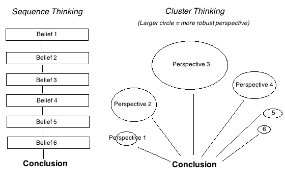
- Sequence better for idea generation
- Cluster better for reaching good conclusions
Why cluster thinking?
- Sequence thinking can go badly wrong with one small mistake
- Successful prediction models (in finance, political forecasting, etc.) use a more cluster-like model
- Aggregated expert opinion is more reliable than individual experts
- Prevents problems arising from impaired judgment
- If you're drunk, take precautions to avoid falling for faulty sequential reasoning
- Historical cases of violent fanaticism arose from sequence thinking; cluster thinking puts more weight on the "don't hurt people" rule
- When uncertainty is high, unknown unknowns likely dominate the impacts of our actions
- Expert opinion predicts which way the arguments I haven't thought of yet will point
- The bulk of impact from donations comes from unknown flow-through effects
- Market efficiency
http://blog.givewell.org/2013/05/02/broad-market-efficiency/
- We expect good opportunities to be found already, which is reason to be skeptical of apparent promising interventions
- Encourages more exploration over exploitation
- EAs tend to be too quick to dismiss large areas as unworthy of exploration
Advantages of sequence thinking
- The world needs more sequence thinking more than it needs more cluster thinking
- Sufficiently robust sequences strongly inform the output of cluster thinking
- Some conclusions (developing-world interventions > developed, GCRs matter a lot) originally struck me as naive chains of logic but which were more thoroughly researched than I at first believed
- Better at generating creative and unconventional ideas
- More transparent and easier to discuss the inputs
- Cost-effectiveness analyses have helped by forcing us to reflect on our views
- Can lead to deeper understanding of a subject
- Must make good predictions about multiple links in a chain of reasoning
Cluter thinking and argumentation
- Cluster thinkers often offer limited arguments that don't reflect all their reasoning; transparency is harder than with sequence thinking
- Instead of asking whether a sequence argument has explicit problems, ask how much uncertainty there is and see if other arguments reach the same conclusion
- I take arguments for developing-world interventions > developed-world more seriously after learning that other people I respect agree, developing-world charites have more robust evidence
The balance I try to strike
- Sequence thinking generates more novel ideas; novel ideas are usually wrong but often useful
- Supporting an org based on novel ideas is valuable if it has high learning value
- I often change behavior to get benefits of supporting an idea but don't follow it fully (e.g. donate lots of income but not so much that you are the best person to spend marginal dollars on)
MD Thoughts
- Holden (and maybe GW in general) is too reliant on cluster thinking in ways that get him stuck on ideas that are fairly obviously wrong. I can see the case that GCRs are highly speculative and we need to research them better. But he supported developed-world interventions for too long in early GW history when it was pretty clear that developing-world interventions are way better, and he continues to undervalue nonhuman animals, possibly because the conclusion that they matter a lot derives from sequence thinking and doesn't fulfill clustery parameters like "most people care about this problem" (although it should for him still fulfill "lots of people I respect care about this problem").
- Cluster thinking has problems such as overweighting many weak arguments versus one strong argument. For example, for vegetarianism, you can make a list of arguments like "it's healthier" and "factory farm workers are mistreated" and most people interpret these as linearly increasing the strength of the argument, even though these don't matter that much. They're not weak in the sense of being likely to be wrong, but in the sense that they're not as important.
Finance Shorts finance
Warren Buffett's portfolio is explained as 0.3% annual alpha + 0.98 beta + 0.00 SMB + 0.31 HML - 0.10 UMD + 0.15 BAB + 0.44 QMJ
Those are the coefficients for Berkshire's 13F portfolio. Berkshire itself had more alpha for reasons that are unclear to me (I didn't read the paper).
Frazzini, Kabiller & Pedersen (2013). Buffett's Alpha. Table 4.
Ranking of techniques to reduce trading costs: banding (holding positions for longer before selling) > reducing rebalancing frequency >> trading only cheap-to-trade securities
Novy-Marx, R., & Velikov, M. (2019). Comparing Cost-Mitigation Techniques.
Andrew Wellington: We looked at news from times when value stocks switched from underperforming to outperforming and even with perfect hindsight, we couldn't find anything in the news that triggered the switch
from Value After Hours S7E8
Commodity open interest significantly increased around 2005

Trendfollowing performance got worse at around the same time, although this would only explain performance within commodities, and it doesn't explain strong performance in 2008 and 2022
Vanguard funds pass 100% of securities lending profit to investors (after paying program costs) funds
from Rational Reminder Podcast #368: Jim Rowley & Andy Maack
me: 2015–2025 VOO beat SPY by 8 bps per year (source)
Since inception, QVAL/IVAL outperformed the 2% Net indexes by ~1.5%pp, and VMOT outperformed the 2% Net index by ~0.5%pp funds
This suggests that real-world fees are substantially lower than 2%


Data quality improvements to Fama-French factors made Beta and HML larger, and SMB smaller
If a factor is data mined, you should expect it to get smaller after improving your data. This is a way of getting "out-of-sample" evidence
source: Production of U.S. Rm-Rf, SMB, and HML in the Fama-French Data Library
Asness: Ask The Audience only works when people can't talk to each other. If they can talk, the crowd becomes a mob
from Meb Faber Show #527
Corey Hoffstein: asset class trends might happen because there's hardly any money correcting asset-class mispricings
https://twitter.com/choffstein/status/1775924815032975378
> Samuelson’s dictum argues that the market is micro efficient but macro inefficient. There are a lot of people trying to pick stocks… but where’s the capital balancing global equity and bond exposure? (Certainly not in the target date fund programs!)
Corey also says about the "trend is counter-hedge" theory:
> You certainly could [argue the other direction]. Which would, arguably, fall more in the behavioral camp as “non-profit seeking traders” pushing prices further in the same direction. > > They’re all just theories as to why trends emerge. There is no definitive data supporting any of them, in my opinion.
In 39 developed countries 1841 to 2019, stocks lost to inflation in 12% of 30-year periods.
Anarkulova, Cederburg & O'Doherty (2021). Stocks for the Long Run? Evidence from a Broad Sample of Developed Markets.
Morgan Housel: A lot of finance consists of very educated people being shocked when something that's consistently happened for hundreds of years happens again.
https://twitter.com/morganhousel/status/1548776359404523520
Most of the time someone says "unprecedented volatility" there is, in fact, precedent, from like two years ago or less.
Commodity momentum tends to buy backwardation and short contango commodities momentum
Miffre & Rallis (2007). Momentum Strategies in Commodity Futures Markets
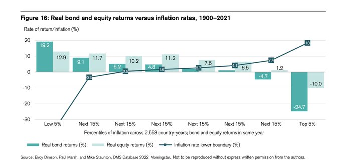
SBF on distinguishing good and bad trades
(based on in-person conversation)
- It's hard
- Understand why the opportunity exists and who's on the other side
- We usually do arbitrage trades where the downside is easy to see and you can figure out if it's worth it
- We also do directional bets
- A lot of our trades are based on instinct that we've developed over time
Jeffrey Ptak: Funds with a 40% annual return for 5 years earned an average of –5.7% per year over the subsequent 5-year period
https://twitter.com/syouth1/status/1473831880218787846
- One fund (Voya Russia) earned >40% for 39 different 5-year periods ending 2003 to 2008, but never performed >40% again
A stock's ask order depth is far higher at the 52 week high than at any other time. momentum
Vedova et al. (2021). Liquidity and Price Impact at the 52 Week High
B/M predicts stock return, but correlation with HML does NOT predict stock return. factors
Daniel & Titman (1998). Characteristics or Covariances?
James O'Shaughnessy took FCF/EV as second best value factor. Meb says it's "basically the same thing" as SHYLD
- This corroborates my findings that FCF behaves similarly to dividends, and it makes logical sense
Jason Calacanis (on Meb Faber show?): SeedInvest and Republic are the only good equity crowdfunding platforms
- Syndicates are ok but equity crowdfunding without syndicates is a negative signal
Lu Zhang on Behind the Markets: momentum anomaly is stronger in developed markets than emerging markets
- This goes against the behavioral explanation of momentum because you'd expect emerging markets to have more unsophisticated investors with behavioral biases and less "smart money" exploiting them
Wes Gray: CAPE doesn't help much with tactial asset allocation; use pure trend-following instead.
Source: The Investor's Podcast #123 Part 2- Momentum Investing w/ Dr. Wesley Gray. 8min.
His reasoning is that CAPE does work long-term, but you could end up spending several years sitting in cash while the market makes big returns, and you don't want to do that.
Things quant trading firms/HFTs can do
- Buy/short ETFs that deviate from NAV
- Arbitrage mispriced derivatives (e.g. instrument price is $X but derivative has implied price $X+0.001)
- Trade based on news
- Trade against retail investors by buying order flow from brokerages
- This (take the opposite side when the market suddenly demands liquidity at any price) > its cute how people think the top-tier quant firms do complicated nonlinear machine learning models on satellite imagery or whatever when they're actually just really good at being the offer you lift $10 over market
- Intra-day mean reversion (Cliff Asness says this is probably still a big part of what they do) -2025-09-06
Startup probability of exit by round
| Source | Seed | A | B | C | D |
|---|---|---|---|---|---|
| Dealroom | 7 | 12 | 18 | 22 | 29 |
| CB Insights | 29 | 33 | 29 | 21 |
- CB Insights data is inferred–could be wrong, and susceptible to rounding errors
- A TechCrunch article gives related info but doesn't directly answer the question
- I saw something a while ago suggesting P(Exit) stays around 0.3, but now I can't find it
Health & Fitness Shorts fitness health
When is blood pressure too low?
- Hypotension is defined as blood pressure below 90/60. It is usually not harmful but it can cause symptoms like dizziness, nausea, or headaches (source)
- Journal of Hypertension 2023 guidelines say < 120/80 is "optimal". No level is described as too low
- RCT: Intensive treatment to get blood pressure below 120 reduced all-cause mortality (especially cardiovascular) by more than standard treatment to get BP below 140. But intensive treatment caused higher rates of some adverse events
The biggest health difference between tofu and whole soy is that tofu has less fiber. Both are rich in isoflavones but the exact nutrient composition varies.
One study found that tofu contains some isoflavones in a more bioavailable form; a different study found that isoflavones are more bioavailable in boiled edamame.
summary source: Gemini Deep Research https://gemini.google.com/app/e393af01d52df1b0
And tofu has more fat and less carbs (source: the nutrition label), which is better for me personally since my diet has plenty of sources of carbs but not as much fat.
Nuckols: My read of the literature is that being physically active (step count) causally predicts longevity even if you exercise.
Stronger by Science Podcast: Walking Benefits and Pre-Sleep Protein @ 32 min
All-cause mortality is minimized at an iron intake between 11 and 14 mg.
Yang, C., Hu, T., Li, C., & Gong, A. (2024). Dietary iron intake predicts all-cause and cardiovascular mortality in patients with diabetes.
There are no clear health differences between runners of 10Ks, half-marathons, and marathons/ultra-marathons
Wirnitzer, K., Boldt, P., Wirnitzer, G., Leitzmann, C., Tanous, D., Motevalli, M., Rosemann, T. et al. (2022). Health status of recreational runners over 10-km up to ultra-marathon distance based on data of the NURMI Study Step 2.
Take zinc if you have a cold
[Cochrane review] Nault, D., Machingo, T. A., Shipper, A. G., Antiporta, D. A., Hamel, C., Nourouzpour, S., Konstantinidis, M. et al. (2024). Zinc for prevention and treatment of the common cold.
1g/day vitamin C reduces severity of the common cold
Hemilä, H., & Chalker, E. (2023). Vitamin C reduces the severity of common colds: a meta-analysis.
Tendons and ligaments don't have their own blood supply. They absorb/release fluid every time they relax/contract, so you need to move them to recover them
source: Mitch Hooper https://www.youtube.com/watch?v=9NPo5CN6bWY
"Turns out once you have enough leucine in a meal, any extra is pointless"
"and tastes like vile Satan's asshole" -Dr. Mike https://www.youtube.com/watch?v=80plw6FQzfg&t=11h35s
Hammer curls work the brachialis more, which should contribute to bicep peak shape
Jeff Nippard, The Best and Worst Biceps Exercises
Sitting is fine if you're physically active
Sandbakk, S. B., Nauman, J., Zisko, N., Sandbakk, Ø., Aspvik, N. P., Stensvold, D., & Wisløff, U. (2016). Sedentary Time, Cardiorespiratory Fitness, and Cardiovascular Risk Factor Clustering in Older Adults–the Generation 100 Study.
Interventions can have smaller effects on mortality than on lesser outcomes
Context: I was confused by Cochrane review on saturated fat which found a bigger effect on CVD events than on CVD mortality, intuitively the effect on mortality should be bigger because interventions have bigger impacts on unhealthier people. But the below exercise meta-analyses found the same pattern (and with better p-values) that mortality has a smaller RR than the lesser outcome.
Maybe this happens because some (eg) CVD events are minor and easy to prevent, and the ones that kill you are big and hard to prevent, so a minor intervention is more likely to prevent a minor event than a major event.
- Effect of Exercise on Mortality and Recurrence in Patients With Cancer: A Systematic Review and Meta-Analysis found RR = 0.76 with exercise and cancer mortality, and RR = 0.52 with exercise and cancer recurrence
- Efficacy of exercise-based cardiac rehabilitation post–myocardial infarction: A systematic review and meta-analysis of randomized controlled trials found RR = 0.74 with all-cause mortality, RR = 0.64 with cardiac mortality, and RR = 0.53 with heart attack
Henselmans: Trained individuals probably don't have a higher protein requirement in an energy deficit because that would be a triple interaction effect
https://www.youtube.com/watch?v=__hRCUDVJx0
- Studies on untrained individuals show no protein requirement <> energy deficit relationship
- Limited research on trained individuals supports this result
- me: This is different from saying that (e.g.) marginal exercise improves health more among high-BMI individuals because that's combining multiple single-interaction effects. If you combine three interactions that don't all have effects individually, it's surprising if a new effect emerges from their combination
Henselmans: CNS fatigue happens to the motor neurons near the muscles that are used. Studies do not find non-local fatigue.
https://www.youtube.com/watch?v=fIcJhKnwp50
- A study found that squat, bench, and deadlift all caused similar amounts of CNS fatigue
- The things that cause local CNS fatigue are the same things that cause muscle fatigue
- Doing squats does not make you physically worse at bicep curls. If your biceps feel weaker, it's due to psychological fatigue, not CNS fatigue
Mixed evidence on whether stress can cause ulcers
sources taken from NYT article Does Stress Cause Ulcers? Here's What Evidence Suggests
- 2015 Danish observational study found people in top third of self-reported stress were 2x as likely to develop ulcers as bottom third over 11–12 years. Odds ratio of 1.19 per point on the 10-point stress scale (p < .001). After adjusting for confounders, odds ratio decreased to 1.11 per point (p < .001). Psychological Stress Increases Risk for Peptic Ulcer, Regardless of Helicobacter pylori Infection or Use of Nonsteroidal Anti-inflammatory Drugs
- 2015 Korean observational study found no association between stress and ulcers (p = 0.862), but did find an association between stress and IBS (p < .001) and reflux esophagitis (p < .001), see Table 2. The Effect of Emotional Stress and Depression on the Prevalence of Digestive Diseases
- My weak conclusion: the claim "stress can cause ulcers" may be true but it's definitely unproven
"Metabolically healthy obesity" is still associated with increased health risks
https://www.redpenreviews.org/reviews/everything-fat-loss/ referenced meta-analyses: CVD, atherosclerosis, NAFLD, kidney function, diabetes
BBM regarding Peter Attia's Outlive
I have actually familiarized myself with a fair amount of the ideas and recommendations he's made in his book, due to a number of questions I've received on the topic. I found the injury-related content to be, by far, the worst. Whereas he actually seems to be quite vigilant about being evidence-based in the realm of cardiovascular disease, for example, all of this seems to go completely out the window in the realm of pain and injury management/"prevention". The vast majority of claims made in that context are simply made up, or repeated from "experts" he's listened to … who similarly made these claims up.
gnuckols: I've never been able to PR squat and deadlift at the same time. I can PR one while the other is on maintenance volume.
from Stronger By Science podcast: exercise technique and minimum effective dose training
AHA recommends getting no more than 6% of calories from added sugar
https://www.heart.org/en/healthy-living/healthy-eating/eat-smart/sugar/added-sugars
- 6% = 43 grams on maintenance and 36 grams when cutting
- Clif Builder Bar plus 400 calories chocolate-covered almonds = 42 grams
- SKP = 32 grams
BBM: Hadza hunter-gatherers have same % calories from sugar as westerners, but almost no diabetes
from #290: Reaction to Huberman's Back Pain Podcast and April 2024 Research Review
Optimal plant protein combinations for DIAAS (for age 6mo–3y)
- pea/wheat 60/40: 85
- pea/wheat/soy 25/20/55: 90
- soy/wheat 90/10: 90
- soy/oat 90/10: 92
- potato + almost any plant protein gets a DIAAS >= 100
- yeast: 97 ([[https://www.ncbi.nlm.nih.gov/pmc/articles/PMC9654170/]])
BBM: Professional runners might only do interval sprints every 2 weeks. You don't need to do them once or twice a week.
Most people do their easy conditioning too hard and their hard conditioning too easy. If you enjoy your HIIT, it's too easy. But you don't have to do it every week.
from #270: Sydney Q&A Part II
Smoothies retain nutrients and fiber.
- Castillejo, N., Martínez-Hernández, G. B., Gómez, P. A., Artés, F., & Artés-Hernández, F. (2015). Red fresh vegetables smoothies with extended shelf life as an innovative source of health-promoting compounds.
- Chu, J., Igbetar, B. D., & Orfila, C. (2017). Fibrous Cellular Structures are Found in a Commercial Fruit Smoothie and Remain Intact during Simulated Digestion.
When you're at high body fat, your body puts on muscle even in a deficit. So you don't lose much by doing a mini-cut in the middle of a bulk
Eric Helms interview with Mike Israetel https://www.youtube.com/watch?v=q1J3WGz_QJU
BBM: A 2x BW squat is not meaningfully better for health than 1.5x
Podcast #280: Great Debates in Fitness and Health #4, Part 1
BBM: Compared to calorie restriction, exercise disproportionately causes one to lose visceral fat (organ fat), which is the worst kind of fat 
Podcast #258: Dec 2023 research review. Abdominal aerobic endurance exercise reveals spot reduction exists: A randomized controlled trial.
BBM: Blood iron level is not a good indicator of anemia. best indicator is ferritin. you probably want over 50; under 20 is definitely iron deficient
Podcast #241: Anemia
By one measure, 80-year olds who strength train are as strong as untrained 30-year olds. fitness
.jpeg)
Source: Kenney, Wilmore & Costil (2015). Physiology of Sport and Exercise.
Glycemic index doesn't really matter health
Cochrane (2023). Do low glycaemic index or low glycaemic load diets help people with overweight or obesity to lose weight?
> Low glycaemic index or glycaemic load diets probably result in little to no difference in change in body weight [compared to higher glycaemic index diets or any other diets].
Resistance training is associated with reduced all-cause mortality up to 140 minutes per week, but more training is associated with increased all-cause mortality (in older subjects). fitness health
https://www.strongerbyscience.com/research-spotlight-lifting-longevity/
Momma et al. (2022). Muscle-strengthening activities are associated with lower risk and mortality in major non-communicable diseases: a systematic review and meta-analysis of cohort studies
For more, see [2023-07-06 Thu] Nuckols: What is the optimal dose of resistance training for longevity?
A twin study found that sun exposure accelerates apparent aging, and sunscreen mitigates this health
Guyuron et al. (2009). Factors contributing to the facial aging of identical twins.
RCT with some weird effects on CO2 and cognition health
Subjects performed worse on cognitive tasks at 1200 ppm than 600 ppm, but performed better at 2500 and 5000 ppm
Soy protein is probably as good as whey protein fitness health
Barbell Medicine: Our measure of protein quality which measures digestibility multiplied by content of the limiting amino acid (tryptophan/methionine):
whey soy pea wheat gluten 1.0 0.99 0.89 0.25 - One experiment found that omnivores vs. vegans who supplemented whey protein vs. soy protein and followed a supervised lower-body strength program showed equal strength gains. Hevia-Larrain et al. (2021), "High-Protein Plant-Based Diet Versus a Protein-Matched Omnivorous Diet to Support Resistance Training Adaptations: A Comparison Between Habitual Vegans and Omnivore"
- Study was on novices so probably doesn't mean much
- Soy has ~70% as much essential amino acid content as % of total protein compared to whey. Gorissen et al. (2018), Protein content and amino acid composition of commercially available plant-based protein isolates
Lab mice have plausibly not been getting fatter health
https://twitter.com/natalia__coelho/status/1521205212802859008?s=20&t=yvfdVKYOb3f1AaPcz3jtqQ
epistemic note: the evidence is weak on both sides, the situation hasn't gotten much scrutiny
How much should you update on a COVID test result? health
https://www.lesswrong.com/posts/cEohkb9mqbc3JwSLW/how-much-should-you-update-on-a-covid-test-result
A rapid antigen test has a Bayes factor of 100x–200x. Therefore, if you don't have symptoms or any prior reason to expect you have COVID, there's likely a <10% chance that you actually have it. If you have symptoms, it's highly likely that you do in fact have COVID.
(Given my lifestyle, I'm assuming a <0.1% prior probability that I have COVID at any given time)
45% of whole wheat protein is fully digested, compared to >90% in wheat protein isolate health
"Ingestion of Wheat Protein Increases In Vivo Muscle Protein Synthesis Rates in Healthy Older Men in a Randomized Trial" https://www.ncbi.nlm.nih.gov/pubmed/27440260
Caffeine health
https://examine.com/supplements/caffeine/
- Increases power output at doses >5mg/kg (which would be ~450mg for me)
Effects of chewing gum health
(source: Wikipedia)
- Chewing improves cognitive function but also impairs it by being distracting. On net, people perform cognitively best just after they have stopped chewing gum; effect lasts 15-20 minutes.
- Chewing sugar-free gum reduces cavities
- especially when sweetened with xylitol which inhibits the growth of certain cavity-causing bacteria
- especially when chewed just after eating
- Has unclear effects on stomach; could reduce acid reflux but could also cause ulcers
Resistance training is associated with decreased mortality even after adjusting for cardiorespiratory fitness. health
https://www.bmj.com/content/370/bmj.m2031 http://www.ncbi.nlm.nih.gov/pubmed/18595904 http://startingstrength.com/articles/barbell_medicine_sullivan.pdf
resistance training has 1/3 the effect size of cardio (hazard ratios 0.91 and 0.69), and the combined effect (0.58) is larger than the effect from multiplying the two hazard ratios
Of people who intentionally lose 10% of their body weight, 30% of them maintain the full weight loss for five years and 50% retain half the weight loss. health
http://ajcn.nutrition.org/content/74/5/579.short
- According to Alyya Leib on Facebook (a nutrition masters student), this meta-analysis shows 50% success rate for 2 years, but at 5 years out, there's only a 5–20% success rate [citation needed]
Listening to relaxing classical music for 45 minutes before going to bed improves sleep quality. health
Harmat, L., Takacs, J., & Bodizs, R. (2008). Music improves sleep quality in students. Journal of advanced nursing, 62(3), 327-335. http://onlinelibrary.wiley.com/doi/10.1111/j.1365-2648.2008.04602.x/abstract
Facts & Research Shorts research
Andrew Gelman on the state of academic psychology psychology
- People can write papers where the abstract contradicts the title and get 100 citations and nobody notices https://statmodeling.stat.columbia.edu/2018/04/06/important-distinction-truth-evidence/
- People (i.e. Dan Gilbert) can say "psychology has a ~100% replication rate" in a Harvard PR piece and the PR person doesn't notice. They would probably notice if a Harvard biologist said "creationism is true" https://statmodeling.stat.columbia.edu/2016/10/20/we-have-a-ways-to-go-in-communicating-the-replication-crisis/
IRS audits people with >$10M income ~50x as much as people with under $100K finance taxes
https://www.irs.gov/pub/irs-utl/statement-for-updated-audit-rates-ty-19.pdf
rate for people under $100K is ~0.2%, >$10M is 2.0%
IQ is important psychology
- Gottfredson (1997). Why g Matters: The Complexity of Everyday Life.
- Reeve & Charles (2008). Survey of opinions on the primacy of g and the social consequences of ability testing: A comparison of expert and non-expert views.
- Note: This survey isn't as high quality as eg IGM Panel, but it's the best survey I'm aware of
Selected items with mean agreement score and percentage who agree (4 or 5 on a 1 to 5 scale):
Item Mean %A g is measured reasonably well by standardized tests 4.5 97 g enhances performance in all domains of work 4.3 97 g is the most important trait determinant of job performance 4.3 93 g tests are fair 4.0 77 Using cognitive tests leads to more social justice than their abandonment 4.0 73
In a regression where X and Y are on the same scale, the slope equals the correlation math
More generally, \(\beta = r \cdot \displaystyle\frac{\text{SD}(Y)}{\text{SD}(X)}\)
It has been claimed that people falsely remember speculation as factual, but one experiment found the opposite psychology
https://psycnet.apa.org/record/2021-90808-001 "In case of doubt for the speculation?" (2022)
People work shorter hours than they think career
https://www.bls.gov/opub/mlr/2011/06/art3full.pdf
- Men who estimated 70+ work hours per week and women who estimated 60+ work hours were off by 25 hours
- People who worked <60 hours were off by 5-10 hours
- People's estimates of time spent on all activites add up to >168 hours
- People overestimated housework by a factor of two
Tumblr's adult content ban was responsible for approximately a 30% reduction in site activity.
"Counterfactual" because activity was already declining, but it declined much faster following the ban.
You only need to test with 5 users career
https://www.nngroup.com/articles/why-you-only-need-to-test-with-5-users/
- Number of problems found follows an exponential distribution, where a single test user will find about 1/3 of design problems. That means you only need 5 test users to find 80% of design problems
Lots of bankers went to prison for the financial crisis
www.bloombergview.com/articles/2015-09-11/prosecution-policies-and-worried-unicorns

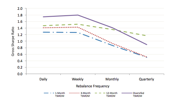
On average, a voter in America has a 1 in 60 million chance of being decisive in the presidential election.
Andrew Gelman, Nate Silver, and Aaron Edlin (2012). "What is the probability your vote will make a difference?" http://www.stat.columbia.edu/~gelman/research/published/probdecisive2.pdf
Simpson's Paradox: Americans do worse on education (PISA) scores than many other countries, but when we break America into ethnic groups, each ethnic group scores better than its origin country.
http://isteve.blogspot.com/2013/12/pisa-reading-scores-by-race-america.html research by Steve Sailer
A car probably costs about $700 a month to own, so it's worth spending about $700/month more on an apartment that's closer to work.
- But you can probably reduce this figure by buying a cheaper car
Statistical prediction rules out-perform expert human judgments
http://lesswrong.com/lw/3gv/statistical_prediction_rules_outperform_expert/
- Example: [rate of lovemaking] - [rate of fighting] reliably predicts marital happiness
- When experts are given access to SPRs, they still underperform the SPRs themselves
You don't know why you make the choices you do. psychology
http://lesswrong.com/lw/6p6/the_limits_of_introspection/ (Lots of specific evidence presented in the article)
SAT predictive power
SAT I scores have ~r=0.05 with Freshman GPA. High school GPA and SAT II scores both have ~r=0.25.
"UC and the SAT: Predictive Validity and Differential Impact of the SAT I and SAT II at the University of California" http://www.tandfonline.com/doi/abs/10.1207/S15326977EA0801_01
- Note: This study only covered the UC schools and it's only one study, not a review. And it's from 2002.
- 2022-08-07: At any particular school, SAT scores should have no correlation with GPA because it's being selected on. Same reason why reading and math SAT scores appear anticorrelated
Related: https://www.lesswrong.com/posts/GQLmPpf9Wava6BTXJ/the-irrelevance-of-test-scores-is-greatly-exaggerated
SAT correlates with intelligence at r=0.5 to r=0.9
Frey (2019), "What We Know, Are Still Getting Wrong, and Have Yet to Learn about the Relationships among the SAT, Intelligence and Achievement" https://www.ncbi.nlm.nih.gov/pmc/articles/PMC6963451/
People most highly rate your social attractiveness when you have ~300 FB friends.
http://www.psychologytoday.com/blog/psyched/200901/facebook-friends-too-many-too-few Tong, S., Van Der Heide, B., Langwell, L., & Walther, J. (2008). Too Much of a Good Thing? The Relationship Between Number of Friends and Interpersonal Impressions on Facebook
Things that replicated, but that you're misinterpreting
People would rather shock themselves than be alone with their thoughts
- https://twitter.com/juliagalef/status/1467967241815691264
- > On average, people in the "electric shock" study rated thinking as ~somewhat enjoyable. And that statement is true even just for the subset of people who chose to shock themselves. / Most people who chose to shock themselves said they did it just because they were curious
- http://datacolada.org/25
- https://www.newyorker.com/tech/annals-of-technology/thinking-alone
Things that didn't replicate
See also big lists of psychology replications: https://forrt.org/reversals/ (more comprehensive) https://aethermug.com/posts/famous-cognitive-psychology-experiments-that-failed-to-replicate (focused more on famous experiments)
Putting a pencil in your mouth makes you happy
it did replicate actually, it's just a weak effect.
Coles, N. A., Larsen, J. T., & Lench, H. C. (2019). A meta-analysis of the facial feedback literature: Effects of facial feedback on emotional experience are small and variable.
Stanford Prison Experiment
see BBC replication
Hard-to-read fonts make you more analytical
Meyer, Frederick, Burnham et al. (2015). "Disfluent Fonts Don't Help People Solve Math Problems." digitalcommons.chapman.edu/cgi/viewcontent.cgi?article=1095&context=esipubs
Implicit association tests
Blanton et al. (2009). Strong Claims and Weak Evidence: Reassessing the Predictive Validity of the IAT. http://www.law.virginia.edu/pdf/faculty/reassessingpredictivevalidityoftheiat.pdf [meta-analysis]
Ego depletion (?)
response to judge parole lunch study: http://www.pnas.org/content/108/42/E833.long
see also http://daniellakens.blogspot.com.au/2017/07/impossibly-hungry-judges.html
and http://journal.sjdm.org/16/16823/jdm16823.html
A recent pre-registered succesfully replicated ego depletion: http://sci-hub.tw/https://doi.org/10.1016/j.jesp.2018.01.005
Name bias in resumes/applications
https://www.ucas.com/file/74801/download?token=M80wi05k
Summary comment: "None of the six projects produced conclusive evidence that masking applicants’ names led to significantly different admissions outcomes". The final recommendation is that "introducing a provider-wide name-blind process could incur significant cost, which may be difficult to justify given the lack of evidence about its value in widening participation and access."
Stereotype threat (?)
- https://replicationindex.wordpress.com/tag/stereotype-threat-and-womens-math-performance/
- more recent experiment: https://www.tandfonline.com/doi/full/10.1080/23743603.2018.1559647
- meta-analysis found no significant effect after adjusting for publication bias. Flore, P. C., & Wicherts, J. M. (2015). Does stereotype threat influence performance of girls in stereotyped domains? A meta-analysis.
- look at this nasty disgusting funnel plot. it's literally the example used on the Wikipedia page for publication bias
- look at this nasty disgusting funnel plot. it's literally the example used on the Wikipedia page for publication bias
- 2021 meta-analysis did find a significant effect: Effectiveness of stereotype threat interventions: A meta-analytic review
Dentists are named Dennis
http://andrewgelman.com/2011/02/09/dennis_the_dent/
2022-12-26: This is not actually a rebuttal of occupational nominative determinism, just a link to a paper rebutting it, to which Gelman has no apparent opinion. Comments have some discussion between the original paper authors.
Bystander effect
"Would I be Helped? Cross-National CCTV Footage Shows That Intervention Is the Norm in Public Conflicts" https://psyarxiv.com/nqscj/
- In CCTV footage, bystanders are observed to help 90% of the time, and probability increases with the number of bystanders
Dunning Kruger effect
Nuhfer, Edward; (retired), California State University; Cogan, Christopher; Fleischer, Steven; Gaze, Eric; Wirth, Karl (2016). "Random Number Simulations Reveal How Random Noise Affects the Measurements and Graphical Portrayals of Self-Assessed Competency."
Nudges (?)
Maier, Bartos, Stanley & Wagenmakers (2022). "No evidence for nudging after adjusting for publication bias." https://www.pnas.org/doi/full/10.1073/pnas.2200300119
- This paper uses complicated statistics so idk if it's legit
- They define "nudge" broadly. The narrower thing of "people stick with the default" might hold up
Lottery winners and paraplegics are equally happy a few years later
Dan Luu's take: https://danluu.com/dunning-kruger/
(this didn't actually not replicate, it was just never shown in the first place, much like Dunning Kruger)
Lottery winners are happier. Oswald & Winkelmann (2019), Lottery Wins and Satisfaction: Overturning Brickman in Modern Longitudinal Data on Germany; Kim & Oswald (2020), Happy Lottery Winners and Lottery-Ticket Bias; Gardner & Oswald (2007), Money and mental wellbeing: a longitudinal study of medium-sized lottery wins.
Chess grandmasters can't memorize random positions faster than beginners
Dan Luu: https://danluu.com/dunning-kruger/
the original paper purporting to show this had N=1 (one grandmaster vs. one novice). failed to replicate in Gobet and Simon, in "Recall of rapidly presented random chess positions is a function of skill"
Created: 2026-04-10 Fri 16:35