Cross-posted to the Effective Altruism Forum.

Last updated 2020-05-17.

Summary

Philanthropic investors probably have greater risk tolerance than self-interested ones. Altruists can use leverage—borrowing money to invest—to increase the expected utility of their portfolios. They may wish to lever their portfolios at much higher ratios than self-interested investors—likely 2:1 to 3:1, and perhaps much higher (practical concerns notwithstanding).

Unlike normal investors, altruists care about reducing their correlations with other investors, so they should heavily tilt their portfolios toward uncorrelated assets.

This essay will discuss:

Traditional vs. altruistic investing
Basic arguments for using leverage
Appropriate levels of risk for altruists
The importance of uncorrelated assets, and where investors might be able to find them
Potential changes for philanthropic behavior

Disclaimer: This should not be taken as investment advice. This content is for informational purposes only. Any given portfolio results are hypothetical and do not represent returns achieved by an actual investor.

Summary
Contents
Glossary
Introduction
Risk aversion for altruistic causes
Risk aversion for altruists
Donors can decrease correlation
Return expectations
How should this change philanthropists’ behavior?
Conclusion
Notes

Glossary

This essay uses a number of terms that may appear unfamiliar. I define most terms when I first use them, but this section provides an easy reference.

$\boldsymbol\eta$ (eta): A numeric value for relative risk aversion that determines the shape of an agent’s utility function.

$\eta = 0$ implies a linear utility function, that is, no diminishing marginal utility.
$\eta = 1$ implies logarithmic utility, which is the value most often used in theoretical models.
$\eta > 1$ implies sub-logarithmic utility, which empirically describes most individuals’ preferences.

Cash: For our purposes, cash does not refer to currency, but to an investment that’s considered safe, such as short-term US Treasury bills. See “Risk-free rate.”

Isoelastic utility function: A utility function that exhibits constant relative risk aversion. If someone has an isoelastic utility function, their risk aversion does not change based on how much money they have.

The isoelastic utility function is defined by

\begin{align} \displaystyle \begin{cases}{\frac {c^{1-\eta }-1}{1-\eta }} & \eta \neq 1 \\ \ln(c) & \eta =1\end{cases} \end{align}

where $c$ is consumption and $\eta$ is a shape parameter.

Leverage: The process of borrowing money in order to invest more than 100% of one’s assets.

Marginal utility: Utility gained when someone gains a new good or service. For our purposes, we care about the marginal utility of money: how much utility a person gains from an extra dollar.

Relative risk aversion (RRA): The extent to which an agent favors safe bets over risky ones. See the definition of $\eta$.

Risk-free rate: The interest rate investors can earn without taking on any risk, such as the rate earned by short-term US Treasury bills.

Samuelson share (S): The proportion of someone’s portfolio they invest in a risky asset.

If $S = 1$, they invest their entire portfolio in the asset.
If $S < 1$, they invest $S$ of their portfolio in the asset and the rest in cash.
If $S > 1$, they use leverage to invest more than 100% of their portfolio in the asset.

Utility function: A function that assigns a real number to how much an agent values each possible outcome. In our case, a utility function takes in an amount of money and returns the utility of having that much money.

Introduction

What makes altruistic investing different from traditional investing?

For the most part, altruists and traditional investors have the same incentives regarding how they should invest—they want to invest in the portfolio with the best return for an acceptable level of risk. Altruists and self-interested investors differ in two key ways:

Charitable causes probably have slower-diminishing marginal utility of money than individuals, so altruists should seek greater risk.
Self-interested people only care about how much money they have, while altruists care about how much money all other (value-aligned) altruists have.

And arguably a third way (more on this later):

Traditional individuals avoid certain market-beating factors like value and momentum for reasons that aren’t captured by a standard utility function, and altruists do not share these reasons.

Regarding the first two differences between altruists and other investors:

The first difference means altruists should be willing to use more leverage than individuals, to the extent that their marginal utility diminishes more slowly.
The second difference implies that altruists who are thoughtful about investing should not proportionally invest their money in the optimal portfolio; instead, they should attempt to push the overall pool of value-aligned philanthropic money in the direction of optimal.

Improving on conventional investing wisdom

In Common Investing Mistakes in the Effective Altruism Community, Ben Todd describes some ways people can improve their investment decisions over the status quo. Before considering leverage, investors should understand and implement these suggestions.

My essay will assume that readers agree with Todd’s section 3, “Not being diversified enough.” Quoting the most relevant portion:

Many people I’ve spoken to are almost fully invested in US equities. I think the rationale for this is that equities have been the best returning asset historically, so there’s no reason to own anything else. Another rationale is that since you can’t beat the market, you should put everything into equities.

But US stocks do not equal “the market”. If you try to tally up all global financial assets, you get something like this:
18% US stocks
13% Foreign developed stocks
5% Foreign emerging stocks
20% Global corporate bonds
14% 30 year bonds
14% 10 year foreign bonds
2% TIPs
5% REITs
5% commodities
5% gold
This represents the truly agnostic portfolio. If you think you have no ability the beat the market, then this is the portfolio with the best risk-return. 100% US equities is a huge bet on just one asset.

From 1973 to 2013, a portfolio like this returned 9.9% per year. In comparison, stocks returned 10.2%. So you only gave up a tiny 0.3% to switch to this portfolio.

In return, you had far lower risk. The volatility of the 100% equity portfolio was 15.6%, whereas this diversified portfolio had a volatility of only 8%. The maximum drawdown was also only -27% compared to -51% with equities. The wide diversification also makes you less vulnerable to unforeseen tail risks.

The much lower volatility means you could have levered up 2x and ended up with the same amount of volatility and same drawdowns as equities, but returns that were twice as high, at 20% per year.

Additionally, I would recommend readers review Todd’s section 6, “Not beating the market”:

Most people I speak to are sold on the “expert common sense” view that amateur investors shouldn’t try to beat the market, and should instead invest in index funds. I basically agree with this view. However, if you’ve got a little more time to put into investing, I think it’s worth considering the idea of tilting your investments towards assets that have value (are cheap based on metrics like P/E and P/B), high momentum (have gone up in the last 12 months, are above their 200-day moving average) and low volatility. If you do this within equities, I think it’s possible to beat the market by a couple of percentage points.

Most people are skeptical when I claim that value and momentum investing beat the market, as I believe they ought to be. Justifying this claim against the efficient market hypothesis requires a high burden of proof. I cannot meet this burden in only a few paragraphs, so I will refer to some longer writings on the subject for anyone still curious.

Asness et al. (2013) Value and Momentum Everywhere examines eight asset classes (US stocks, UK stocks, continental European stocks, Japanese stocks, country equity index futures, government bonds, currencies, and commodity futures) and finds that value and momentum work in all eight.

Two additional papers: Fact, Fiction and Momentum Investing; and Fact, Fiction and Value Investing. Targeted at skeptics, these articles offer high-level summaries and refer to other academic papers that provide evidence for the efficacy of momentum and value.

The books Quantitative Value and Quantitative Momentum, the first by Wesley Gray and Tobias Carlisle, and the second by Wesley Gray and Jack Vogel, discuss value and momentum, respectively. These books discuss why value and momentum work and how the authors believe the strategies can best be implemented. For readers specifically interested in whether or how it is possible to beat the market, I believe Quantitative Momentum gives a more concise and better-reasoned explanation, particularly in the first two chapters.

One could argue that individuals should not avoid value and momentum and behave irrationally by doing so. I mostly agree with this, but individuals do have valid reasons for wanting to avoid value and momentum—they can underperform the broad market for long stretches of time, which many people may find undesirable for various reasons:

They care about maintaining social status, and thus are risk averse not only with respect to losing money, but also with respect to losing money relative to their peers.
For professional investors, relative (but not absolute) underperformance can cause them to lose clients.

Altruists should not consider these compelling reasons to avoid market-beating strategies and should make efforts to sidestep the behavioral biases that lead people to avoid them.

Risk and leverage for traditional investors

According to standard economic theory, individuals have some level of risk tolerance that dictates how much risk they are willing to take on their investments. For our purposes, we can assume that individuals have some isoelastic utility function, which means there exists a constant $\eta$ > 0 describing someone’s relative risk aversion (RRA), and their utility function is given by:

\begin{align} \displaystyle \begin{cases}{\frac {c^{1-\eta }-1}{1-\eta }} & \eta \neq 1 \\ \ln(c) & \eta =1\end{cases} \end{align}

An $\eta$ of 0 corresponds to linear marginal utility of money (that is, no diminishing marginal utility). $\eta$ = 1 indicates logarithmic utility, while $\eta$ > 1 gives sub-logarithmic utility. Different individuals report substantially different RRAs, and different methods of empirically determining $\eta$ give different results; but most people appear to have $\eta$ values ranging from 1 to 4¹.

$\eta$ can be used to determine how much risk someone is willing to take on an investment. For simplicity, suppose only two investments exist: a risk-free investment and a risky one. (The risky investment might not be a single asset, but a diversified combination of stocks and bonds.) Let $R_f$ be the rate of return of the risk-free investment, and let the risky investment follow a log-normal distribution parameterized by $\mu$ and $\sigma$: that is, the logarithm of the distribution is a normal distribution with mean $\mu$ and standard deviation $\sigma$.

Let Alice be an investor with RRA equal to $\eta$. Alice can invest some proportion of her portfolio into her risky asset; Ayres and Nalebuff in their book Lifecycle Investing refer to this proportion as the Samuelson share.

Under traditional model assumptions, the optimal Samuelson share is given by $S = \displaystyle\frac{\mu - R_f}{\sigma^2 \eta}$. If S < 1, Alice should put the rest of her money into the risk-free asset; if S > 1, she should use leverage to invest more than 100% of her portfolio.²³

For most reasonable assumptions about future stock returns and for typical values of $\eta$, S < 1. That is, most people do not want to invest more than 100% into stocks.

However, Ayres and Nalebuff argue in Lifecycle Investing that people should treat their future income as an asset in their portfolio. Because young people will have much more money in the future than they do today, they should use leverage to diversify their investments across time. If you expect that 90% of your investable earnings lie in the future and you have all your current investments in stocks, your portfolio is effectively 10% stocks/90% future-earnings. If instead you get 2:1 leverage, you now have 20% in stocks and 80% in future earnings, which is more reasonable than 10%/90%. (Arguably you should have something like 5:1 leverage so that your portfolio contains half stocks and half future earnings; but that much leverage brings additional complications, so Ayres and Nalebuff only recommend going up to 2:1.)

Risk aversion for altruistic causes

What RRA ($\eta$) should we use for charitable causes and how does it compare to individuals’ RRAs? This is a complex question and I cannot offer a complete answer within the scope of this essay. People often assume that altruists’ utility functions lie somewhere between logarithmic and linear ($0 < \eta \le 1$); e.g., Paul Christiano wrote, “I think logarithmic returns are fairly conservative for altruistic projects […], and that for most causes the payoffs are much more risk-neutral than that.” I consider this a reasonable assumption, but the question deserves more investigation. A full analysis is out of scope, but I will briefly model how utility might diminish for three of the most popular cause areas in effective altruism: global poverty, farm animal welfare, and existential risk.

Global poverty

In the long run, marginal utility for philanthropists cannot diminish any faster than the rate of the self-interested individual with the slowest-diminishing utility curve. If some person has a lower $\eta$ than everyone else, once everyone’s welfare has been improved to the point where that person has the greatest marginal utility of money, (which might take a long time, but in theory will happen eventually), philanthropists cannot do worse than to simply give their money directly to that person.

But the person with the steepest utility curve might not currently have the highest marginal utility of money, because there probably exist many other worse-off people who need money more. We care about how philanthropists should invest their money right now, which means we want to know what the utility curve of global poverty interventions currently looks like.

GiveWell rates GiveDirectly as one of the top charities working on global poverty. GiveDirectly simply gives cash directly to the world’s poorest people. GiveWell believes cash transfers do not represent the most cost-effective global poverty intervention, but that they probably aren’t much worse than the best interventions. And we can analyze GiveDirectly’s marginal utility easily because we can model its value in terms of the utility curves of the people receiving the cash. So for now, let’s assume GiveDirectly represents the pinnacle of global poverty charities.

For simplicity, let’s assume GiveDirectly has no overhead costs and give the world’s poorest people money without encountering any obstacles. GiveDirectly’s goal is to provide as much utility to as many people as possible by increasing their wealth and thus allowing them to buy more stuff that makes their lives better—that is, GiveDirectly wants to maximize the aggregated individual consumption utility function:

\begin{align} \displaystyle\sum_1^n u_i(C(i)) \end{align}

where $i$ represents the $i^{th}$ person, $C(i)$ is the consumption level of the $i^{th}$ person, and $u_i()$ gives the utility function over consumption for the $i^{th}$ person. (Note that this aggregate utility function is almost certainly not isoelastic, which means we cannot assign it a relative risk aversion parameter $\eta$.)

GiveDirectly’s mathematically-optimal strategy—assuming all individuals have the same value of $\eta$ (which is false, but a common simplifying assumption in development economics)—is to give cash to the world’s poorest person until they have as much money as the second-poorest person; then give cash to the bottom two poorest people until they reach the level of the third-poorest person, and so on.

The world’s poorest person and the world’s millionth-poorest person have almost the same amount of money, so giving a dollar to the latter does almost as much good as giving a dollar to the former. The world contains many more poor people than GiveDirectly can afford to help, so (given our simplifying assumptions) cash transfers have nearly linear marginal utility of money, at least for donors with less than a few hundred billion dollars⁴.

We had to make several simplifying assumptions to reach this conclusion. I cannot say with confidence that the conclusion holds in the real world, but it does seem plausible that this simplified model roughly describes how the global poverty cause operates in terms of its diminishing marginal utility:

In practice, GiveDirectly can give money only to people it can reach; but it can reach such a large set of people that this does not substantially affect its rate of diminishing utility.
GiveDirectly’s overhead costs scale sub-linearly with money donated⁵, so they don’t cause the utility curve to fall off more rapidly.

Interventions that GiveWell considers more cost-effective than cash transfers, such as deworming, probably experience more rapidly diminishing marginal utility. Or, as GiveWell might say, these interventions have less funding capacity than cash transfers do. Let’s call these “superior” interventions, in the sense that they are superior to cash transfers. We can determine the rate of diminishing by answering three questions:

How much better are superior global poverty interventions than cash transfers?
How much philanthropic money has already gone into superior global poverty interventions?
How much money would need to flow into global poverty before all superior interventions became fully funded?

I don’t know the answers to any of these questions, but let’s make up some on-the-face plausible answers and see what we get.

GiveWell’s cost-effectiveness analysis gives an answer for the first question: GiveWell estimates that its top charities do between 5 and 60 times as much good as GiveDirectly.⁶ The 60x charity is an outlier and GiveWell’s estimate might not be accurate, so let’s suppose the current best charity is 10x as cost-effective as cash transfers.
The USAID budget is $40 billion. We can extrapolate this to perhaps $200 billion per year in global spending, and maybe $10 trillion in the past few decades. Prior to a few decades ago, GDPs were low enough and global poverty spending was unpopular enough that, for the sake of this rough estimate, we can assume prior spending was $0. Of this $10 trillion, maybe $1 trillion is spent effectively. (One could probably come up with a much better estimate with a few hours of research.)
In 2018, GiveWell moved $111 million to top charities other than GiveDirectly (see GiveWell Metrics Report) and moved similar amounts in 2015–2017. GiveWell probably can keep moving money for a while, and its top charities only represent a fraction of better-than-cash-transfers giving opportunities—we should include effectively-utilized money from other philanthropic organizations such as the Gates Foundation. So philanthropists can spend perhaps $100 billion before running out of such opportunities.

Assign the answers to these questions to symbols $b$, $m$, and $m'$, respectively. The value of $\eta$ is given by⁷

\begin{align} \eta = \displaystyle\frac{\log b}{\log (1 + m’ / m)} \end{align}

For the given values of $b$ = 10, $m$ = $1 trillion, and $m'$ = $100 billion, we get $\eta$ = 24, which indicates remarkably high risk aversion (most individuals have an RRA between 1 and 4¹). This implies that the 100 billionth dollar spent on global poverty did $10^{24}$ times as much good as the trillionth dollar, which seems highly implausible.

If instead we assume that global poverty interventions can absorb a full $1 trillion, we get a relative risk aversion of 3.3. Perhaps we also believe that few organizations spent their money ineffectively, and only $100 billion went to effective causes, which means over 90% of the value of superior global poverty interventions has yet to be captured; giving $\eta$ = 1.

Alternatively, we could ask what proportion $p$ of superior giving opportunities philanthropists have funded already. This proportion equals $\displaystyle\frac{m}{m + m'}$, so in the first set of numbers given, this would equal $1 trillion / $1.1 trillion = 0.91.

My intuition suggests that philanthropists have used up most of the superior opportunities, yet they still need much more funding to exhaust them—I would guess we are substantially less than 90% of the way there. (Some people who reviewed this essay had the opposite intuition—that the majority of superior opportunities have yet to be filled.) I do not have any particular expertise on this issue and find a wide range of answers plausible, which means $\eta$ could plausibly take on many values. But it does seem unlikely that cash transfers would have a much smaller $\eta$ than self-interested people’s, while other global poverty interventions would have a much larger $\eta$.

To view from another angle, and pump intuitions in a different way: How much money do we believe superior interventions can absorb relative to cash transfers? I would guess that superior interventions can absorb close to as much funding as cash transfers (to within a factor of two), which suggests that the two $\eta$s cannot differ by much.

It might make more sense to model superior giving opportunities using a non-isoelastic utility curve (i.e., the value of $\eta$ is not fixed). This would violate many of the assumptions in this section, requiring much more analysis.

Ultimately, my weakly-informed guess is that superior global poverty interventions experience diminishing marginal utility at a slightly but not much higher rate than cash transfers.

Farm animal welfare

If we wish to fund interventions that attempt to reduce the incidence of factory farming or improve farm animals’ well-being, what diminishing marginal utility might we expect these interventions to experience?

We can think about farm animal welfare as an extension of global poverty in at least two different ways, each of which results in a different model and a different answer for $\eta$.

The first way: We can consider factory farming interventions in the same way we examined superior global poverty interventions. Some amount of money has been spent on preventing factory farming; and some additional amount of money can be spent before efforts on farm animal welfare are no more cost-effective than cash transfers. We can answer the same three questions we raised in the previous section and find the value of $\eta$ for factory farming interventions.

We probably believe that the best farm animal interventions are more cost-effective than the top global poverty interventions, meaning we assign a greater value to $b$. All else equal, a larger $b$ results in a larger $\eta$—that is, greater risk aversion.

Pushing in the other direction, probably only a small fraction of value in the anti-factory-farming space has been captured already, which means the proportion $p = \frac{m}{m + m'}$ is small.

Some example values:

if $b = 100$ and $p = 1/2$, then $\eta = 6.6$
if $b = 100$ and $p = 1/10$, then $\eta = 2$
if $b = 100$ and $p = 1/100$, then $\eta = 1$
if $b = 10$ and $p = 1/1000$, then $\eta = 0.33$

The second way: When considering cash transfers, we looked at how much money it would take to improve the station of the N worst-off people so that they become as well off as the (N+1)^th-worst off person. We can extend this model by looking at a set of sentient beings including both humans and factory-farmed animals (and naturally we could extend this to include other beings as well, but for now let’s just consider those two categories). As a weird but useful and sort-of-correct abstraction, assume factory-farmed animals consume money in the same way that humans do, but that they’re really, really poor, so they have extremely high marginal utility of money. Then philanthropists should give money to help animals until all the animals are as well off as globally poor humans. According to this model, donations to farmed animal welfare have nearly linear marginal utility.

This model seems plausible in some respects, but the first model requires unreasonably small values of $b$ and/or $p$ to produce a similar answer. Both of these models have several obvious shortcomings. They are only meant to be a rough start, not a definitive answer.

Existential risk

Work on existential risk reduction often involves doing research: exploring ways of neutralizing engineered super-viruses, studying how to create stable AI systems, etc. Other types of work can be done, but I will focus on research for now.

Effective researchers begin by focusing on the most promising potential directions. As funding for a field increases, researchers begin pursuing less promising avenues. How quickly does the value of research diminish?

Owen Cotton-Barratt claims in an article, The Law of Logarithmic Returns, that the returns to research grow logarithmically with resources invested. He refers to Nicholas Rescher’s book Scientific Progress: “starting with the observation that progress (counted in terms of the number of “first rate” discoveries) goes linearly with time while resources increase exponentially, [Rescher] deduces that the underlying behaviour is a logarithmic return to resources.” Cotton-Barratt presents some additional empirical evidence suggesting that returns to research scale logarithmically. His follow-up article, Theory Behind Logarithmic Returns, provides theoretical justification for this observation.

Additionally, I spoke with some people involved in existential risk research, and they (independently) agreed that research probably produces logarithmic returns.

Logarithmic returns entail $\eta = 1$. Investors with logarithmic utility have greater risk tolerance than most individual investors by a factor of perhaps 1.5 to 4, but still much less risk tolerance than someone with near-linear utility (such as a donor to GiveDirectly).

Note that this applies to any research-based cause, which could include potential existential risks such as AI safety, biosecurity, and climate change, but also can include other cause areas such as disease prevention, macroeconomic policy, and anti-aging.

Risk aversion for altruists

Uncorrelated small donors are nearly risk-neutral

Suppose you are a philanthropist with a relatively small amount of money, and your investments have no correlation with other philanthropists’. (This second assumption rarely holds true in practice, but let’s take it as a given for now.) If you want to donate to a cause that already has much more money than you do, you have nearly linear marginal utility of money, which means you should behave nearly risk-neutrally.

As a numerical example, let’s say your preferred cause area has $1 billion in funding and you currently have $1 million. Further suppose that this cause has logarithmic utility of money, which means $1 billion produces log(1 billion) = 20.723 utils (where a util is an abstract measurement of utility). If you add your $1 million, your cause now gets log(1,001,000,000) = 20.724 utils, giving (approximately) an extra .001 utils.

If the cause as a whole doubles its funding to $2 billion, the utility will increase from 20.723 to 21.416—so the first $1 billion is worth far more than the second billion. If you double your $1 million to $2 million, the utility of the cause increases to 20.725. Your first million provides .001 utils, and your second million provides an additional .001 utils. The second million does provide less value, but only slightly less—if we use more significant figures, we can see that the first million gives .00999 utils and the second million gives .00998.

To look at it another way, suppose you have the choice between getting either (A) $X with certainty, or (B) 50% chance of getting $2 million and 50% of getting nothing. At what value of X are you indifferent between A and B? Most self-interested people would probably say something in the range of $50,000 to $300,000, with some people going somewhat higher or lower.⁸ But in this example, your value of X would be $999,500.

How risk-averse are large donors?

While uncorrelated small donors experience nearly linear marginal utility of money, large donors do not. For our purposes, a large donor is one who can fund a significant fraction of their preferred cause area. A donor who is the sole funder of a cause experiences diminishing marginal utility at the same rate as the cause itself, as discussed in Risk aversion for altruistic causes.

Correlated small donors look like large donors

Unlike individual investors, small donors do not care only about how their own portfolios perform. Altruists who want their causes to receive more funding also want fellow donors’ investments to perform well.

Quoting Paul Christiano:

[T]he fact that I am a small piece of the charitable donations to a cause shouldn’t matter. My risk is well-correlated with the risk of other investors, and if I lose 10% of my money in a year, other investors will also lose 10% of their money, and less money will be available for charitable giving. This holds regardless of whether a cause has a million donors or just one.

In effect, many small donors with highly correlated investments have similar risk preferences to a single large investor.

Time diversification

The book Lifecycle Investing explains the concept of time diversification (an excerpt from the first chapter, which introduces the concept, is available online). The basic idea: Treat your future income as an asset in your investment portfolio. Suppose you have $10,000 in investments and expect to invest an additional $90,000 of your earnings over the next 20 years. In that case, you have invested only 10% of your lifetime savings. If you invest in a standard 60% stocks/40% bonds portfolio, you will have $6,000 in stocks today but $60,000 by the time you retire (adjusted for inflation and market returns). That means you have much more exposure to market fluctuations in 2040 than in 2020. You can solve this by diversifying across time: applying leverage to your current $10,000 portfolio while holding more bonds or cash in 2040.

The principle of time diversification applies to philanthropists as well, in two different ways:

You should consider the donations you can make with your future income.
The future might contain more value-aligned altruists who will increase the size of the philanthropic money pool.

Lifecycle Investing provides information on how to determine optimal leverage at each point in time given various assumptions, particularly in chapters 3 and 4.

According to Lifecycle Investing, investors should calculate their optimal Samuelson share. Then they should consider the discounted present value of their future income as an asset in their portfolio, and hold stocks in the correct proportion of their lifetime portfolio. For example, an investor with $10,000 in stocks and $90,000 in discounted future earnings⁹, and with a Samuelson share of 0.6, should ideally hold 60% in stocks. Therefore, they should theoretically invest with 6:1 leverage to get their stock holding up to $60,000. Their overall portfolio would then look like this:

 $60,000 stocks
-$50,000 debt
 $90,000 future cash

which can be simplified to

 $60,000 stocks
 $40,000 cash

giving the investor their desired portfolio.

Similarly, if you are the sole funder of a cause, you currently have $10 million, and you expect the cause’s funding in the future to increase to $30 million in present-value dollars, then you can treat that extra $20 million as cash in your portfolio, and increase your current portfolio’s risk by 3x. If you have a Samuelson share of 1, increase your risky holdings from 100% to 300% (that is, 3:1 leverage); at a Samuelson share of 0.5, increase risky holdings from 50% to 150%.

For already-popular causes such as global poverty, we might expect future funding to continue increasing at the historical rate. If global poverty donations grow with GDP, we should treat this as a bond in the global poverty investment portfolio that pays the GDP growth rate in interest. Assuming $20 billion in annual effectively-directed global poverty donations (from the rough estimate given above) and 1% real GDP growth, we can treat global poverty donations as a $2 trillion asset that grows at 1% real per year and has the same risk level as GDP growth. If we look only at the GiveWell money moved of ~$100 million and assume it will grow with GDP (historically it has grown faster than that), this suggests we treat future GiveWell donations as an asset worth $10 billion.

Many causes that effective altruists prioritize do not see much mainstream interest, but might expect to get much more interest in the future. For example, a few years ago, AI safety had hardly any funding, but recently has been growing in popularity. For such causes, philanthropic investors may wish to substantially lever up their portfolios to create time diversification. But also consider that if future funding looks uncertain, investors may wish to take on less risk.

Adjusting for other altruists’ investing behavior

Suppose there exist two risky assets A and B. Almost all investors invest in A, and hardly anyone invests in B, but both provide similar risk-adjusted return. An ordinary investor should maximally diversify by splitting their assets into approximately half A, half B.

Altruists care how much money other value-aligned altruists have. As discussed above, they wish to reduce their assets’ correlation with other altruists’, not just with their own. Therefore, the optimal allocation would not be 50% A/50% B, but perhaps 100% B. If most people heavily overweight asset A, then an investment-minded philanthropist can move the “altruistic portfolio” closer to optimal by investing only in B.

Additionally, the pool of philanthropic money has some optimal Samuelson share. If the aggregate altruistic portfolio does not reach that risk target, then thoughtful investors can compensate by over-leveraging to make up for others’ insufficient leverage. (If most altruists take on too much risk, one can compensate by holding extra cash, but this seems unlikely in practice.)

These considerations matter a great deal. If your portfolio only makes up a small part of the altruistic portfolio, this suggests that you should hold no conventional assets and instead invest your entire portfolio in something weird-looking in order to maximize uncorrelated return. It also might mean you should take on a huge amount of leverage and incur a near-certain probability of bankrupting the altruistic portion of your portfolio in order to increase the overall risk and return of the altruistic money pool.

Ideally, altruists would agree about optimal investment choices. Suppose Alice invests in 100% US equities while Bob goes 100% short on US equities. If they share values, they have a mutual interest in ensuring that the other invests optimally. One of them must be making a mistake, so they should come to an agreement about how they both should invest. Insofar as it is possible, rather than unilaterally attempting to shift the altruistic money pool, we should cooperate with other philanthropists and come to a consensus on how to invest.

Although most altruists do not diversify well or take on enough risk, it is plausible that large philanthropists—who hold a disproportionate share of the altruistic money—invest better. Investment-minded altruists should particularly care about how large donors invest. If they already invest optimally, that means small donors have less of a reason to try to shift the overall investment pool.

What if RRA varies over time?

If a philanthropist’s utility curve does not follow the isoelastic utility function defined above, they do not have a single fixed value of $\eta$. If $\eta$ increases or decreases over time, we cannot simply look at the optimal amount of investment risk to use at a particular point in time and then maintain it forever. Furthermore, we do not necessarily want to vary leverage over time based on the value of $\eta$.

First, some simplifying assumptions:

You will invest your money until time $t$, at which point you will donate it. Let $\eta_t$ be your RRA at this time. You will donate all your money at once, rather than donating over time according to some schedule.
You do not have enough money to meaningfully shift the utility curve, so the value of $\eta_t$ does not change as a result of your donation.
You know the optimal time $t$ to donate. (In actuality, the optimal value of $t$ depends on the shape of the utility curve, so we cannot know it without first knowing $\eta_t$.)

Under these assumptions, the marginal utility of your donation depends only on $\eta_t$, not on the value of $\eta$ at any other time. $\eta_t$ determines the relative risk aversion of your donation, which means it tells you how much risk you should take on. The desired level of risk is given by the Samuelson share formula:

\begin{align} S = \displaystyle\frac{\mu - R_f}{\sigma^2 \eta_t} \end{align}

(Recall that $\mu$ = expected return of investment, $\sigma$ = standard deviation, and $R_f$ = risk-free rate.)

Donors can decrease correlation

Because most donors’ investments are correlated, their utility curves fall off more rapidly than if they were independent. But it is not destined to be this way.

If correlated donors experience logarithmic (or worse) marginal utility and uncorrelated (small) donors experience nearly linear marginal utility, donors should care a lot about finding uncorrelated sources of income.

What sorts of uncorrelated assets can we find, and what rate of return can we expect from them? In this section, I will survey a few asset classes worth considering. This is not meant to be an exhaustive list, nor will I describe in detail the pros and cons of each; this list is just meant as a starting point. For more on some of these diversifiers, see AQR (2018), It Was the Worst of Times: Diversification During a Century of Drawdowns.

Note that if all altruists started investing in these diversifying asset classes, they would no longer provide as substantial diversification benefits. But I don’t expect that to happen in the near future.

(Individual investors should care just as much about decreasing correlation by diversifying. The difference is that ordinary investors can simply hold an optimal portfolio; but altruists care about other altruists’ money, so they may want to overweight diversifiers relative to what an individual investor would do.)

Bonds

Historically, bonds have had near-zero correlation to stocks (even anti-correlation at times). Most investors already hold bonds as well as stocks, however, so adding bonds to our portfolio does not do much to reduce our correlation to other donors.

Commodities

Fewer donors invest in commodities. Commodities provide low correlations to stocks (but usually still positive), and by carefully selecting good investment vehicles, they can provide positive (but probably not great) return. For more, see Levine et al. (2016), Commodities for the Long Run.

Managed futures (trendfollowing)

A better idea than bonds or commodities might be managed futures. These are actively-managed long/short strategies that intend to provide uncorrelated returns. Managed futures funds usually use trendfollowing: going long on assets that have been trending upward over a certain time horizon, and going short on assets that have been trending downward. When I discuss managed futures in this essay, I am talking specifically about ones that use trendfollowing strategies.

Hurst et al. found promising results in Demystifying Managed Futures (2013). According to a backtest described in the paper, a diversified managed futures strategy (investing across stocks, bonds, commodities, and currencies) produced a return of 19.4% with a standard deviation of 10.8%, and an alpha over stock, bond, and commodity indexes of 17.4% (figure 2, page 49). That is, the managed futures strategy produced a 17.4% return that was not explained by the return of stocks, bonds, or commodities. This suggests that managed futures provide a strong uncorrelated source of returns not captured by most investors.

I highly doubt that actual investors can realize a risk-adjusted return as high as what the Hurst paper found in its backtest, but I do expect managed futures strategies to be worth pursuing in some circumstances. For more on how managed futures strategies behave and why they might provide alpha, see the paper. And for further evidence, see Hurst et al. (2014), A Century of Evidence on Trend-Following Investing, which tests managed futures trendfollowing strategies going back to 1880.

Going forward, I expect managed futures to perform worse for three primary reasons:

The 19.4% figure does not include fund fees or transaction costs.
Managed futures strategies depend on interest rates, which are much lower now than they were over the studied period.
More investors today use managed futures strategies than did in the 80’s, 90’s, or early 00’s. (But note that managed futures strategies have gotten less popular over the past decade.)

At the same time, Hurst et al. offer some reasons to be optimistic about future performance:

Transaction costs have been decreasing over time as markets become more liquid.
Investors have access to markets that were not previously investable, such as emerging market equities and emerging market currencies.
Even assuming muted future returns, trendfollowing still provides valuable diversification.

The paper provides some quantitative analysis on how managed futures benefit a portfolio even if they produce much worse returns than they did historically.

Why do managed futures strategies provide alpha? Why have they not been arbitraged away? The answer is not known for certain, but the most reasonable hypothesis is that the majority of investors avoid it because it can underperform their benchmark for long periods of time. I cannot do this hypothesis justice, but in brief, consider this performance chart of a managed futures mutual fund (EQCHX) compared against the S&P 500 over the five-year period from 2014 to 2019 (the dark blue line is EQCHX and the light blue line is the S&P):

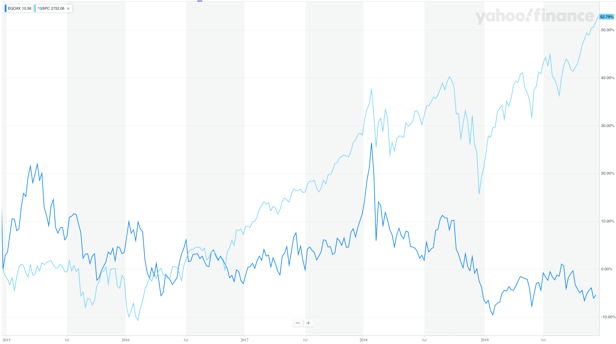
As discussed above, most investors benchmark their returns against an index like the S&P 500, and would be unwilling to suffer five years of dramatic underperformance.

For more on this hypothesis, see Alpha Architect (2015), The Sustainable Active Investing Framework: Simple, But Not Easy.

Will managed futures continue to work? AQR (2018), Trend Following in Focus, discusses this question and concludes that they probably will. In short, managed futures strategies do not appear over-subscribed, and although they have performed poorly over the past few years, similar stretches of poor performance have occurred many times in the past.

Eventually, of course, managed futures strategies will no longer provide uncorrelated returns. (Even if only a small percentage of investors ever adopts such strategies, over time those investors will become richer until they have enough money to eliminate the market inefficiency.) But until then, it appears that small donors with the ability to invest in managed futures can get nearly linear marginal utility of money by doing so.

Buy-and-hold long/short strategies

Altruists might consider pursuing buy-and-hold long/short strategies (as opposed to managed futures, which are actively-traded long/shorts). That is, buy some asset that has moderate but not perfect correlation to what you believe most philanthropists own and short-sell the standard philanthropists’ portfolio. Say you believe all philanthropists put all their money in the S&P 500¹⁰. You could buy a global excluding-US stock market index, which has high but not perfect correlation with the S&P 500, and then short the S&P. As a result, you can get a return stream that’s uncorrelated with other altruistic investors. For example, if the S&P and the global ex-US market are correlated with r=0.8, you could put 500% of your money in the global ex-US market (that is, 5:1 leverage) and short 400% of the S&P 500, for a net 100% market exposure with zero correlation to the S&P. (That is not actually how the math works, but for the purposes of this example, it doesn’t matter.)

At first glance, this seems wasteful: you are shorting an asset that other altruists hold, so your investments cancel each other. But this is still a good idea given the assumption that the S&P-buyers are making a mistake. By using a long/short strategy, you can increase the combined return of all philanthropic money without increasing risk. In other words, you are moving the pool of philanthropic money closer to an optimally-diversified portfolio, and you are doing so more effectively than if you just bought the global ex-US index. Of course, it would be even better to convince other altruists to improve their portfolio holdings.

I suspect (although do not have much evidence) that philanthropists under-weight quite a few asset classes, such as global stocks (especially emerging-market stocks), gold, commodities, and emerging-market bonds. A philanthropic investor might want to buy some of these assets while shorting overweighted ones. An investor might particularly want to do this if they do not believe that managed futures perform as well as I suggested in the previous section.

Note that individual investors would never want to use this sort of strategy. The only reason this type of long/short might make sense is because you believe some investors’ money brings as much value to your utility function as your own money does, but those other investors are under-diversified, so you want to make up for that lack of diversification.

Long/short factor premia

AQR (2018) identified long/short factor premia as the best diversifier according to its backtests. In brief, a long/short factors strategy invests in market-beating factors (such as value and momentum, discussed above) by going long on “good” assets while going short on “bad” assets (according to the factors), producing a market neutral position. For a detailed analysis of this strategy, see Ilmanen et al. (2019), How Do Factor Premia Vary Over Time? A Century of Evidence.

AQR has a Style Premia Alternative Fund (QSPNX) that appears to attempt to follow the strategies identified in Ilmanen et al., although I have only briefly read the fund literature. However, this fund has a $1 million investment minimum, and I am not aware of any similar funds that retail investors can access. The AQR and Ilmanen papers suggest that sufficiently-wealthy altruistic investors may want to invest in a long/short factor fund as a diversifier, and QSPNX might be a reasonable way to do that.

Startups

Another low-correlation investment opportunity, suggested by Paul Christiano:

[I]f you start or invest in a small company, your payoff will depend on that company’s performance (which is typically quite risky but only weakly correlated with the market). […] This special case is only possible because the entrepreneur or investor is putting in their own effort, and moral hazard makes it hard to smooth out all of the risk across a larger pool (though VC funds will invest in many startups). You shouldn’t expect to find a similar situation in investments, except when you are providing insight which you trust but the rest of the market does not (thereby preventing you from insuring against your risk).

Mission hedging

Some altruists have discussed the concept of mission hedging:

How should a foundation whose only mission is to prevent dangerous climate change invest its endowment? Surprisingly, in order to maximize expected utility, it might use ‘mission hedging’ investment principles and invest in fossil fuel stocks. When oil companies perform well (which means they are contributing more to climate change), the anti-climate change foundation will have more money. When more fossil fuels are burned, fossil fuel stocks go up, thus giving the foundation more money. When fewer fossil fuels are burnt and fossil fuels stocks go down, the foundation will have less money, but it does not need the money as much anymore.

A philanthropist could mission hedge and obtain low correlation with other altruistic investors by buying a mission-hedge investment (such as fossil fuel stocks) while simultaneously shorting the broad market. This would not provide ideal diversification because altruists who invest in index funds will still have some exposure to the same risk factors as the long/short mission hedge strategy, but it will reduce correlation.

My impression is that altruistic investors should prioritize maximizing risk-adjusted return, then focus on reducing correlation with other altruists. Mission hedging provides only tertiary value and should be avoided insofar as it impedes the first two goals. But I have not studied mission hedging, and I could be wrong.

What if everyone did this?

If you invest in a particular source of return that’s uncorrelated to the broad market, and many other philanthropists do, too, you have formed a pool of correlated investors, which means your utility curve behaves as if everyone in that pool is a single large donor. Naturally, you would prefer to invest in an asset that’s not correlated with any other altruist’s investments. But an uncorrelated asset with, say, $10 million in philanthropic money still provides much greater marginal utility than the S&P 500, in which orders of magnitude more value-aligned philanthropists already invest.

I doubt that huge sums of philanthropic money will flow into unusual investments like managed futures in the near future, which means those people who do make such investments might experience nearly linear marginal utility of money. That said, most of the arguments in this essay rely on the assumption that the overwhelming majority of altruistic investors will not change their behavior. For the most part, the proposals in this essay eventually will stop being a good idea if enough value-aligned philanthropists adopt them.

Return expectations

The Samuelson share formula requires four parameters: $R_f$, $\mu$, $\sigma$, and $\eta$. We have discussed $\eta$ in some depth, but have not addressed the values of the other three parameters. What might we expect?

Investment firm Research Affiliates (RAFI) publishes an estimate of return expectations based on solid methodology. RAFI updates its predictions regularly based on changing market conditions, but as of this writing, it predicts a 0.4% return after inflation with 14.4% standard deviation for US large-cap stocks over the next 10 years (with a 95% confidence interval of -3.4% to 4.1% return). But of course, investors should diversify beyond US stocks. RAFI estimates that the optimally-diversified portfolio will provide 1.6% real return with 4.0% standard deviation. Investors who hold this portfolio may want to use much more leverage than investors in US stocks, if only because it has a much lower standard deviation. Alternatively, RAFI’s optimal (un-levered) portfolio at the 12% volatility level has 4.5% expected real return; this portfolio has slightly worse return-to-risk ratio (0.375 instead of 0.4), but requires less leverage.

We care about $\mu - R_f$, not just $\mu$. We subtract the risk-free rate $R_f$ because (1) if we hold cash, that cash can earn the risk-free rate; and (2) borrowing money to use leverage requires paying the risk-free rate in interest (at least in theory, see Cost of leverage). Investors can earn $R_f$ without taking on any risk, so in some sense it doesn’t count, and we should subtract it out. The current risk-free rate after inflation nearly equals zero, so we can assume $R_f = 0$ without losing much precision.

As discussed above, investors probably can outperform a fully diversified portfolio by tilting toward value and momentum. Most implementations of value and momentum (such as the Vanguard Value ETF) track a broad market index and only use a weak value or momentum tilt—they have low active share.

What kind of returns might we expect from a high-active-share value/momentum fund? Investment firm Alpha Architect maintains an index it calls the Global Value Momentum Trend Index, investable through the ETF VMOT.¹¹ This index only invests in the top ~5% of stocks matching its criteria. Comparing Alpha Architect’s backtest from 1992 to 2017 against index returns from the Ken French data library, VMOT would have returned 17.4% with a 13.6% standard deviation (before subtracting fees and inflation), versus 9.3%/15.0% for the US + Europe stock markets (which makes for a reasonable benchmark).

For a longer backtest, I attempted to approximate VMOT’s methodology using the Ken French Data Library entries on momentum and value (earnings-to-price), which go back to 1952¹². These data only include US stocks, and we have theoretical reasons to expect the simplified investment strategy represented by these data to (slightly) underperform VMOT¹³. Over the full sample back to 1952, it returned 18.3% with a standard deviation of 16.2%—performing better than in the more recent period. We do not have data on how VMOT might have performed before 1992, but based on results from the Ken French data, it probably would have performed about as well or possibly better than it did in the 1992 to 2017 backtest.

Going forward, we cannot necessarily expect the same returns from a strategy like VMOT. RAFI predicts an average 2.8% return for the global stock market index over the next 10 years. This suggests a differential of 9.3% - 2.8% = 6.5% between historical nominal return and future real return.¹⁴ If we subtract 6.5% from the historical VMOT return, and subtract an additional 2% for fees and costs (which is the figure Alpha Architect uses), we get an 8.9% expected real return for high-conviction value and momentum strategies like VMOT. This is a rough estimate, not an accurate figure. Arguably we should assume value and momentum will not perform as well in the future as they have in the past, and apply an additional discount to this 8.9%. If we discount the excess return by half, we get a 5.9% expected return for VMOT. I will not apply this discount in my calculations, but we should be aware that doing so would change our ultimate estimate of how much leverage to use.

As something of a corroboration, RAFI provides estimates of forward-looking five-year return for various long/short factors. At the time of this writing, it makes the following predictions for its long/short value and momentum factors (net of transaction costs):

5.7% for US large-cap value
1.1% for US large-cap momentum
8.0% for US small-cap value
6.4% for US small-cap momentum

(RAFI’s projections for foreign developed market factors are similar but generally a bit higher.)

A concentrated long-only portfolio on a particular factor would have approximately the same expected return as the long/short factor plus the broad market (although that’s not quite how the math works).

The underlying indexes used by VMOT make some improvements on RAFI’s simple factor model (see Quantitative Value and Quantitative Momentum for details¹⁵), so it might be reasonable to assume a higher expected return for VMOT. If we then subtract fees, we get something close to the original estimate I gave for VMOT (probably a bit higher¹⁶).

RAFI believes the value and momentum premia will work as well in the future as they have in the past, and some of the papers I linked above make similar claims. They offer good support for this claim, but in the interest of conservatism, we could justifiably subtract a couple of percentage points from expected return to account for premium degradation.

Note that RAFI’s estimates use factor timing—attempting to guess how well factors will perform based on the current market environment, rather than just looking at historical behavior. This practice is not widely accepted; for example, see Asness et al.’s Factor Timing is Deceptively Difficult (2017). Also note that these numbers only give expected mean return. Even if these estimates are accurate, we could still see much higher or lower returns due to market volatility.

Uncorrelated returns

As discussed above, altruists have a few options for seeking uncorrelated (or weakly-correlated) returns. Of the (investable) options discussed, managed futures appear best.

The previously-discussed paper A Century of Evidence on Trend-Following Investing found that a diversified managed futures strategy returned 11.2% (nominal) with 9.7% standard deviation over the period 1880 to 2013, after adjusting for estimated fees and transaction costs. As I said above, I do not expect investors to realize returns this high in practice; I would expect a managed futures fund to underperform VMOT after fees and costs, but probably outperform the US stock market on a risk-adjusted basis over the next 10 years. I don’t know much about managed futures—I’ve read a few papers and done some analysis based on AQR’s published data, and that’s my guess based on what I know.

Chesapeake Capital’s managed futures fund (EQCHX), discussed previously, has published performance data (net of fees) going back to 1988. From 1988 to 2020, it returned 9.8% (nominal) with a 19.2% standard deviation. If we subtract inflation and de-leverage to match the risk level of the AQR managed futures strategy, we come up with about a 4% real return with 11% standard deviation.

As discussed in Trend Following in Focus (referenced previously), we have reason to expect managed futures to perform about as well going forward as they did in the past. We don’t know if the 31-year sample for EQCHX is representative of more long-term performance, but it gives a more conservative estimate than the AQR data, so we can use this as a rough projection of future performance. Performance could look dramatically different in the future, but this estimate makes about as much sense as any.

Long-run market return

Market-beating strategies such as value and momentum, and low-correlation, positive-return strategies such as managed futures, almost certainly will perform worse as time goes on. At present, it appears that only a small percentage of investors has high enough tolerance for tracking error to invest in these sorts of strategies. But over time, these investors will become richer and eventually eliminate the market inefficiency.

The Ramsey equation gives the long-run rate of return in an efficient market:

\begin{align} r = \delta + \eta g \end{align}

where:

$r$ = investment rate of return
$\delta$ = pure time preference
$\eta$ = relative risk aversion
$g$ = economic growth rate

This equation holds because individuals discount future money at rate $\delta + \eta g$, so they will require that investments return at least this much; and investments that return more than this will experience inflows until the expected return drops to $r$.

(If historical market returns roughly continue, we can probably expect equities markets to return 3-5% after inflation in the long run.)

An investor maximizes long-run expected utility by, at each point in time, maximizing expected utility for the next point in time¹⁷; and maximizes expected utility at each time step by investing at the level given by the Samuelson share formula based on the expected return $\mu_t$ and standard deviation $\sigma_t$ at each time $t$. Therefore, the long-run expected return does not affect what risk level investors should adopt today.

Caveats

Markets do not behave the way standard theoretical models suggest they do. This section discusses some deviations from theory and how that affects leverage.

Behavior of leveraged investments in practice

Before using leverage, investors should understand how different implementations of leverage can behave in practice. Brian Tomasik’s Should Altruists Leverage Investments? discusses this in detail, with extensive simulations; Colby Davis’s The Line Between Aggressive and Crazy provides a more concise discussion of the most important points. Note that Davis’s article, although it does not say so explicitly, assumes investors have a logarithmic utility function; so some of its conclusions do not apply in the same way for other utility functions. For example, the formula he gives for optimal leverage is a special case of the Samuelson share formula with $\eta = 1$.

Mean reversion

If asset prices follow a random walk, increasing leverage proportionally increases expected value. Unfortunately, prices probably do not (entirely) follow a random walk.

In the short run (on the timescale of days to weeks), stock prices tend to overreact and then mean revert¹⁸. This essentially means that median outcomes happen more often, while high-variance outcomes (where the market goes up and then up again, or down and then down again) occur less often.

As explained by Brian Tomasik, when asset returns are independent across time, leverage proportionally increases mean return, but less-than-proportionally increases (and possibly decreases) median return. Because short-term mean reversion increases the probability of median outcomes, it makes leverage look less appealing.

Additionally, markets exhibit long-run mean reversion over the timescale of years: assets that have gone up (or down) a lot over the past three to five years tend to go down (or up) over the following year. Fortunately, we can adapt to this phenomenon by adjusting our return expectations based on asset valuations, which Research Affiliates does in its estimates that I quoted previously. (Perhaps we could adapt to short-term mean reversion as well, but it would require updating return expectations on a frequent, e.g., daily, basis.)

Assets exhibit medium-term momentum: price trends over the past 6-12 months tend to continue over the next 1-3 months. This works in favor of leverage by increasing the probability of high-variance outcomes while decreasing the frequency of median outcomes.

In summary, there exist three well-established types of price trend: short-term mean reversion, medium-term momentum, and long-term mean reversion. The latter two can work to our advantage (or at least they don’t hurt us), while short-term mean reversion makes leverage look worse. How this affects the value of leverage overall warrants further investigation.

Left skew of investment returns

So far, I have assumed that asset returns follow a log-normal distribution. Asset pricing models traditionally assume log-normal returns, so this assumption has well-established precedent. Unfortunately, it is false.

In practice, asset returns skew to the left: highly negative returns occur more frequently than a log-normal model predicts. Any investor with a concave utility function (i.e., any reasonable investor) dislikes left skew: people disprefer bad outcomes more strongly than they prefer good outcomes. That means investors should take on less risk than log-normal models suggest.

Unpredictability of future return

The Samuelson share formula assumes we know the exact values of forward-looking expected return and volatility. But obviously we don’t. Getting too much leverage generally hurts more than not getting enough, so the more uncertain we are about these parameter values, the less leverage we should want to use (to avoid risking accidentally taking too much risk).

We could account for this by treating mean return and standard deviation as distributions rather than point estimates, and calculating utility-maximizing leverage across the distribution instead of at a single point. This raises a further concern that we don’t even know what distribution the mean and standard deviation have, but at least this gets us closer to an accurate model.

For more, see Chopra, V. K. and W. T. Ziemba (1993). “The effect of errors in mean, variance and co-variance estimates on optimal portfolio choice.”

Cost of leverage

In theory, borrowing money for leverage costs only the risk-free rate. In practice, leverage costs more than that under most circumstances.

Lifecycle Investing recommends buying deep-in-the-money call options. Such options on highly liquid securities tend to cost about the risk-free rate, but options on less-traded securities will carry much higher implicit interest rates.

Investing with margin allows for more flexibility. Interactive Brokers charges the risk free rate plus between 0.3% and 1.5%, depending on the amount of margin used, with higher margin costing lower rates. Investors can use margin to buy any investable asset. Large institutions can potentially negotiate cheaper rates.

Brian Tomasik gives a more thorough survey of types of leverage, along with their advantages and disadvantages.

Higher costs make leverage look somewhat less attractive. We can roughly approximate the impact of a 1% cost over the risk-free rate by subtracting 1% from the expected return of an investment.¹⁹

Taxes

Investors who hold their money in taxable accounts should pay special attention to minimizing taxes. A portfolio that makes frequent trades will incur substantial performance drag due to taxes. (This applies to any investment, not just investment with leverage.)

Taxes reduce expected return, but they also reduce volatility by the same amount. If investors can borrow money for free, they can increase leverage in proportion to the tax rate, which will increase the expected return and standard deviation of their assets by exactly enough to cancel out the tax burden. Unfortunately, investors cannot get free leverage, so taxes will hurt their risk-adjusted return.

Ideally, altruists should invest in tax-sheltered accounts. Foundations can invest however they want, but small donors have more limited options. Donor-advised funds (DAFs) typically only allow a small set of investments. But some funds offer more flexibility in some cases: for example, Fidelity Charitable allows donors with at least $5 million to manage their own investments. It also permits donors with $250,000 to nominate an investment advisor to manage their money. DAFs typically charge 0.6% per year, which substantially hurts your return if you keep money in them for a long time, but this might be preferable to paying taxes every year.

Tax-sensitive investors should prefer ETFs over mutual funds because they do not distribute taxable gains as often. In the long run, an ETF in a taxable account may incur lower costs than a DAF.

This subject deserves much more discussion, and much has been written elsewhere on the subject. Altruists should consider other ways to minimize taxes or, if possible, to invest in tax-sheltered accounts.

Additional caveats

Edward Thorp, The Kelly Criterion in Blackjack Sports Betting, and the Stock Market (p. 32), lists some additional false assumptions of this model:

Stock prices do not change continuously; portfolios can’t be adjusted continuously; transactions are not costless; the borrowing rate is greater than the T-bill rate; the after tax return, if different, needs to be used[.]

How should this change philanthropists’ behavior?

Reasonable leverage ratios (under the theoretical model)

This section ignores all the caveats presented above.

So far, we have arrived at the following conclusions about altruists’ risk preferences:

Uncorrelated small donors experience nearly linear marginal utility of money, regardless of their preferred cause.
Interventions that straightforwardly benefit their recipients, including typical global poverty and farm animal welfare interventions, probably have nearly linear marginal utility; but marginal utility might diminish more rapidly if the best interventions dry up quickly.
Research-based cause areas, including existential risk, probably experience roughly logarithmic marginal utility.

Philanthropists with near-zero risk aversion theoretically maximize the utility of their investments by taking on as much leverage as they feasibly can.

For philanthropists with logarithmic utility—likely including large donors and correlated small donors—the optimal Samuelson share depends on investment return expectations. This table gives Samuelson shares for various investment portfolios, given the return expectations laid out previously. The fourth column $S$ gives desired leverage according to the Samuelson share formula, and the fifth column $S \cdot \mu$ gives expected return after applying leverage. This assumes the real risk-free rate equals 0% (which is approximately true as of this writing).²⁰

Be aware that these estimates depend on assumptions about return expectations that may be false. Furthermore, the estimated optimal leverage only holds under the theoretical model described previously. Although this model is commonly used to approximate investment behavior, it does not accurately reflect real-world trading, for reasons listed in Caveats as well as other reasons.

Investment	$\mu$	$\sigma$	$S$	$S \cdot \mu$
diversified global index, low-vol	1.6%	4%	10.2	16%
diversified global index, high-vol	4.5%	12%	3.4	15%
value/momentum/trend (VMOT)	9%	13%	6.1	55%
managed futures (MF)	4%	11%	3.5	14%
VMOT + MF	7%	10%	7.8	54%

These estimates assume logarithmic utility. If altruists have higher or lower $\eta$, they should prefer lower or higher amounts of leverage (respectively).

Deviations from the theoretical model

On the other hand, a number of caveats reduce how much leverage altruists may want to use. These include market behaviors such as mean reversion, left skew of investment returns, and the unpredictability of future return; as well as practical considerations such as the cost of leverage and taxes.

After accounting for these caveats, large philanthropists or correlated small donors should probably take on more leverage than most individual investors, but substantially less than the numbers given in the previous section. Some have proposed using “half Kelly” instead of the Kelly criterion,²¹ where for our purposes, the Kelly criterion corresponds to $\eta = 1$ and half Kelly means $\eta = 2$. This might roughly account for the various factors that make leverage look less appealing. Or we could look at how historically successful investors have calibrated their risk. For example, Warren Buffett appears to use something similar to the full Kelly criterion, as do many other successful investors.²²

Doubling $\eta$ results in halving $S$ according to the Samuelson share formula. Using the same return estimates as before, this gives $S = 1.7$ for the diversified global index (high-vol) and $S = 4.2$ for VMOT + MF.

Pushing in the other direction, recall that we made two arguments for increasing leverage even further:

Most altruists probably do not take on enough risk, so investment-minded philanthropists should increase leverage to compensate.
According to the principle of time diversification, philanthropists should increase leverage now if they expect their preferred cause area(s) to have greater access to funding in the future.

The first factor weighs overwhelmingly in favor of using leverage for small donors, although not necessarily for large donors (because large donors’ choices more heavily affect the overall altruistic investment pool). The significance of the second factor depends on one’s expectations about future movement growth.

We can never definitively determine the correct amount of leverage to take, and any attempt to model the expected utility of an investment will have many shortcomings. But investors still need to pick a number, even if that number is 1:1 (i.e., no leverage). I do not claim that the leverage ratios offered in this section are optimal—they’re just reasonable guesses based on what I laid out in the previous sections of this essay. Taking too much leverage is worse than not taking enough, so I personally would probably not use this much leverage in practice.

Good Ventures / Open Philanthropy Project

According to many effective altruists’ value systems, most value-aligned money resides with Good Ventures, the foundation that funds the Open Philanthropy Project. Donors should care about how Good Ventures invests its money and about how to adapt their own investments to diversify against Good Ventures. Unfortunately, I do not know how Good Ventures invests, so I have nothing to say about this other than that it matters a lot.

If Good Ventures invests a large portion of its assets in Facebook and does not hedge this investment (which it may or may not do, I don’t know), other philanthropists should pay particular attention to diversifying against Facebook.

Implementation details

I am not an investment professional and do not have sufficient expertise to make a recommendation about how to invest. For informational purposes, I will propose what I believe to be a reasonable and achievable investment plan based on the reasoning laid out in this essay, but with the caveat that a thoughtful investor could likely find a better implementation. This should be considered a best guess, not an endorsement.

First, invest with Interactive Brokers because it offers the cheapest margin rates (at least in the United States²³). Create an altruistic investment account that’s separate from your personal account, because personal accounts should take much less risk.

Second, invest all your altruistic funds into a managed futures fund. As discussed above, philanthropists should care greatly about reducing correlation with other investors; and managed futures look like a particularly promising way of doing that.

I spoke to an investment advisor with knowledge of managed futures, and he suggested AQR Managed Futures Strategy HV Fund (QMHIX) as a good choice. This fund targets high (15%) volatility, which has the dual benefit that (1) investors with high risk tolerance can get higher return with less leverage and (2) the fund produces greater expected return relative to fees. QMHIX is not available to all investors; as an alternative, AXS Chesapeake Strategy Fund (EQCHX)¹¹ has similar methodology, as well as relatively low fees for a managed futures fund.

Third, use as much margin as Interactive Brokers will allow without substantially risking a margin call. Investors using Reg T margin cannot get anywhere close to as much leverage as is theoretically optimal according to the analysis above, so they should get as much as they can. (At least small donors should, to compensate for other donors’ lack of leverage; large philanthropists may want to take less than 2:1 leverage (but perhaps should take more than 2:1; I am uncertain about this).)

Alternative investment strategies

Another similar investment idea: Instead of buying a managed futures fund, buy value and momentum funds while shorting the broad market to produce net zero stock exposure, and then apply lots of leverage. This probably requires portfolio margin rather than Reg T margin, which has certain qualification requirements, so not as many investors will be able to implement this strategy. Some examples of high-conviction value ETFs: IVAL, QVAL, GVAL, SYLD, FYLD, EYLD. And some momentum ETFs: IMOM, QMOM, GMOM.

As a third option, philanthropists could invest in more liquid assets (which would have worse risk-adjusted return) and then use options to get much more leverage. I am inclined to believe that this does not make as much sense. For philanthropists with logarithmic risk aversion, this strategy may result in lower expected utility. Even for those with near-linear marginal utility, using high leverage (say, 10:1 or higher) may impose sufficiently high costs that the resulting investment portfolio will have negative expected return.

Investor psychology

Philanthropists with theoretically high risk tolerance should consider their psychological reaction to pursuing risky and uncorrelated strategies. How will you react if:

you invest your philanthropic money in a risky strategy and lose 90% or more of your money?
you invest in an uncorrelated strategy, and slowly lose money over the course of 5-10 years while most people you know are making money?

Whether a strategy is optimal in theory doesn’t matter if investors can’t follow through with it in practice. I personally do not invest in the manner I described in the previous section; I use something like a combination of that strategy and a more traditional investment portfolio.

Large investors

Sufficiently large investors can non-trivially shift the altruistic money pool by themselves. Rather than investing exclusively in assets with low correlation to other altruists, they should build a well-diversified portfolio with a tilt toward under-weighted asset classes.

Large institutions or ultra high-net-worth individuals most likely can implement a portfolio more effectively than individual investors. They might be able to:

access some types of investments that individual investors cannot (such as long/short factor funds);
hire investment firms to create customized products;
negotiate better margin rates;
use higher leverage ratios.

Wealthy philanthropists or institutions with relatively long time horizons should consider how best to use these advantages.

I would suggest that investors who want additional guidance speak to Alpha Architect. It is an investment management firm that produces high-quality research and investment products (hence why I have cited it repeatedly), and offers custom solutions for large investors. Perhaps more importantly, I believe the owners of the firm genuinely want to help people invest well—an all-too-rare trait among investment managers. The people at Alpha Architect know far more than I do about investing, and likely have better ideas about how to invest in unusual situations.

Conclusion

Confidences

I will conclude by restating the main claims of this essay, with corresponding confidence levels.

On risk and leverage

Highly likely: More altruists should use leverage.

Highly likely: Altruists should consider their own psychology when deciding how to invest.

Likely: Most altruists should have higher risk tolerance than typical self-interested investors.

Likely: The best way to get leverage for most investors is with an Interactive Brokers margin account.

Possible: Many altruists should use as much leverage as they can reasonably manage.

Possible: For most altruists, $0 < \eta \le 1$.

On asset allocation

Highly likely: More altruists should tilt their investments toward value and momentum.

Highly likely: Altruists should pay particular attention to reducing correlation with other altruists’ investments.

Highly likely: There exists a better investment strategy than the one I proposed in Implementation details.

Likely: Altruists should overwhelmingly favor assets with low correlation.

Likely: Altruists should specifically invest in managed futures as a way of reducing correlation.

Possible: Altruists should invest their entire (altruistic) portfolios into managed futures.

Possible: Altruists should specifically invest in any of the funds that I named.

Questions for future consideration

Can we build better models for the utility functions of various causes?
What if we use a utility function with non-constant RRA?
How do effective altruists as a whole currently allocate their investments across asset classes? Which asset classes do altruists under-weight most severely?
How exactly do deviations from the asset pricing model (including left skew and short-term mean reversion) affect desired leverage?
How should one invest if their investment correlation to other altruists lies between 0 and 1?
How should future donations be treated with respect to time diversification? How does the answer vary by cause area?
Should historical donations factor into the utility function? It seems to me that we should count historical good done as part of total utility, but the literature I have read on utility of consumption generally does not do this. Why not?

Acknowledgements

Thanks to Brian Tomasik, Jake McKinnon, Kit Harris, Linda Neavel Dickens, and Michael St. Jules for providing me with valuable feedback. Reviewers do not necessarily endorse any of the claims made in this essay.

Changelog

2020-05-17:

Update managed futures return expectations to incorporate actual historical performance data from managed futures fund EQCHX.
Add a backtest going back to 1952 of a strategy similar to VMOT.

2020-04-29:

Add additional disclaimers.

2020-04-18:

Provide more details and references on managed futures.
Add section on long/short factor strategies.
Miscellaneous small improvements.

2020-01-08:

Add more references to papers on value and momentum that provide further evidence that they work.

Notes

For a short summary of empirical research on people’s risk preferences, see Estimating the Coefficient of Relative Risk Aversion for Consumption. ↩ ↩²
Domian, Racine, and Wilson (2003). Leveraged Stock Portfolios over Long Holding Periods: A Continuous Time Model. ↩
Merton (1969). Lifetime Portfolio Selection Under Uncertainty: The Continuous-Time Case. ↩
Aside: I attempted to write a Python program to determine the marginal utility of cash transfers and at what point risk aversion starts to meaningfully increase. But the program didn’t work very well because, given the way I wrote it, NumPy had to struggle to compute triple-nested integrals far out on the tails of fat-tailed probability distributions. But I only spent a couple of hours on it, so I think such a program should be writable given a more careful approach. ↩
I did not look deeply into this, but GiveDirectly’s staff has not expanded as rapidly as its increase in donations over the past few years, so this statement appears to be true. ↩
GiveWell gave substantially lower numbers in 2018, ranging from 4.2 to 12.2. I have not investigated the reasons for the difference. ↩
Derivation: Marginal utility of the $m^{th}$ dollar is $b$ times greater than the marginal utility of the $(m + m')^{th}$ dollar. The standard isoelastic utility function is defined as

\begin{align} \displaystyle \begin{cases}{\frac {c^{1-\eta }-1}{1-\eta }} & \eta \neq 1 \\ \ln(c) & \eta =1\end{cases} \end{align}

and its derivative is $c^{-\eta}$. The ratio of marginal utilities between $m$ and $m + m'$ should equal $b$:

\begin{align} \displaystyle\frac{m^{-\eta}}{(m + m’)^{-\eta}} = b \end{align}

Solving this equation for $\eta$ gives the desired result. ↩
I estimated this based on a range of typical net worths and relative risk aversions. ↩
This assumes that individuals can treat their future earnings as risk-free. This might not be the case, depending how much volatility one expects in their future career. Lifecycle Investing discusses this more, as well as Milevsky (2012), Are You a Stock or a Bond? ↩
Philanthropists are over-represented in the US, and people in every country over-represent their own country, so it is almost certainly the case that philanthropists over-represent the S&P 500, although obviously they don’t all put all their money in it.

I did a small informal Facebook poll that supports this claim. ↩
Disclaimer: At the time of this writing, I have money invested in this fund. ↩ ↩²
Methodology:
1. Take the top decile by momentum and the top decile by E/P.
2. Create a portfolio weighted 50/50 between these two, rebalanced monthly.
3. Use a combination of the 12-month simple moving average and 12-month time series momentum to risk manage the portfolio, as described by Alpha Architect.
↩
For comparison, the strategy I tested returned 14.4% with standard deviation 16.0% from 1992 to 2017, hypothetically underperforming VMOT by 5 percentage points on a risk-adjusted basis. VMOT makes a number of methodological improvements over the basic strategy I tested, the biggest differences being (1) diversifying internationally, (2) using a value metric that better captures company valuation, and (3) using a more robust risk management methodology. ↩
Does it make sense to treat market factors as additive like this? Yes. The academic literature on finance generally treats factors as additive: see Fama and French (1992), The Cross-Section of Expected Stock Returns. ↩
Any deviations from a well-established investing strategy should raise concerns about data mining. The two books explain why they believe their improvements are not data-mined. They also discuss and reject some alternative potential improvements because they suspect the strategies are data-mined. ↩
Based on my coarse estimate that VMOT has two percentage points higher expected return than the average of RAFI’s eight US+developed large+small value+momentum factors plus market beta, and subtracting VMOT’s fee, we get a 10-11% expected real return. ↩
Proof:
- Characterize investing as a discrete series of time steps from 0 to $\tau$, after which the investor stops investing.
- Each time step has an investment return random variable $r_t$ following a normal distribution parameterized by $\mu_t$ and $\sigma_t$.
- $u(x)$ is the isoelastic utility function, parameterized by some constant $\eta$.
- $S_t$ gives Samuelson share at time $t$ (>1 indicates leverage).
- $x_0$ gives the amount of starting capital.
We wish to maximize expected utility with respect to $S_t$:

\begin{align} E[u(x_0 \exp(\displaystyle\sum_1^\tau r_t S_t))] \end{align}

$u(x)$ is normally defined as $\displaystyle\frac{x^{1-\eta} - 1}{1 - \eta}$. Utility functions are equivalent up to affine transformations, so we can simplify this to $x^{1-\eta}$ (or $\log(x)$ in the case that $\eta$ = 1). For the same reason, we can omit the $x_0$ term. Furthermore, this means the maximum of $S_t$ does not depend on past return, only on the expected distribution of future return.

First, consider the case with only two time steps. Call the leverage-adjusted return in each time step $x$ and $y$.

\begin{align} u(e^{x + y}) = \displaystyle \begin{cases} (e^{x + y})^{1-\eta} = e^{x (1 - \eta)} e^{y (1 - \eta)} & \eta \neq 1 \\ \ln(e^{x + y}) = x + y & \eta = 1 \end{cases} \end{align}

Thus we have:

\begin{align} \displaystyle\begin{cases} u(e^{x + y}) = u(e^x) u(e^y) & \eta \neq 1 \\ u(e^{x + y}) = x + y & \eta = 1 \end{cases} \end{align}

Using the rule determined in the $\eta \ne 1$ case, as well as the fact that $E[X \cdot Y] = E[X] \cdot E[Y]$ when $X$ and $Y$ are independent, we can modify the expected value formula as follows:

\begin{align} E[u(\exp(\displaystyle\sum_1^\tau r_t S_t))] = E[\displaystyle\prod_1^\tau u(e^{r_t S_t})] = \displaystyle\prod_1^\tau E[u(e^{r_t S_t})] \end{align}

This product is maximized with respect to $S_t$ by maximizing each term of the product.

In the $\eta = 1$ case, $E[u(e^{r_1 S(1) + ... + r_\tau S_\tau})] = E[r_1 S(1) + ... + r_\tau S_\tau]$. By linearity of expected value, this equals $E[r_1 S(1)] + ... + E[r_\tau S_\tau]$. This sum is maximized with respect to $S_t$ by maximizing each integral.

Thus, for any value of $\eta$, we maximize long-run expected utility by independently maximizing expected utility at each time step.

Thanks to Michael St. Jules for providing feedback on how to substantially simplify this proof. ↩
De Bondt and Thaler (1985). Does the Stock Market Overreact? ↩
This underestimates the cost of leverage because on a left-skewed distribution, subtracting a constant across multiple time periods reduces the mean by more than that constant. And it overestimates the cost of leverage because fees reduce the volatility of an investment. Whether it under- or over-estimates on net depends on the specific properties of the investment. ↩
Correction 2020-01-20: Originally, I calculated $S$ as $\frac{\mu}{\sigma^2 \eta}$, but technically this is not correct.

Let $\mu$ and $\sigma$ be the mean and standard deviation of the asset, and let $\mu_S$ and $\sigma_S$ be the parameters used in the Samuelson share formula.

The $\mu_S$ parameter in the Samuelson share formula should be the log of the mean, and the $\sigma_S$ parameter should be the standard deviation of the log of the return (where the log of the return is normally distributed). That is:

\begin{align} \mu_S = \log(1 + \mu) \end{align} \begin{align} \sigma_S = \sqrt{\log\left(\displaystyle\frac{\sigma^2}{(1 + \mu)^2} + 1\right)} \end{align}

$\mu_S$ and $\sigma_S$ appproximately equal $\mu$ and $\sigma$, so simply using $\mu_S = \mu$ and $\sigma_S = \sigma$ is not a bad approximation, but it’s not quite accurate.

Thanks to Gordon Irlam for providing this correction. ↩
MacLean, Thorp, and Ziemba (2010). Good and bad properties of the Kelly criterion. ↩
MacLean, Thorp, and Ziemba (2010). The Kelly Capital Growth Investment Criterion: Theory and Practice. Part VI: Evidence of the Use of Kelly Type Strategies by the Great Investors and Others. ↩
Interactive Brokers operates in other countries, but I do not know if other countries have better brokerage firms. ↩

How Much Leverage Should Altruists Use?