The Structural Return Argument Against Value Investing
Value investing had a singularly bad run from 2007 to 2020. (And it hasn’t done great since 2020, either.) Is that because value investing is broken, or did it simply hit a streak of horrendous luck?
Skeptics of value investing have made many claims about why value investing doesn’t work anymore, but these claims tend to be light on evidence.1 Value investing proponents have empirically researched most of these claims and found that they don’t stand up to scrutiny.234
The poor performance of the value factor was not primarily driven by weakening fundamentals, but by the widening of the value spread. A wider value spread makes value investing look more attractive going forward, not less.
What's the value spread?
Value stocks are defined using the ratio of a stock’s price to some fundamental metric—for example, earnings, book value, or cash flow. If we use earnings as the metric, then value stocks are those with low P/E ratios and growth stocks are the ones with high P/Es.
The value spread is the ratio of price-to-fundamental ratios between growth stocks and value stocks. For example, if growth stocks have an average P/E of 30 and value stocks have an average of 15, then the value spread is 30/15 = 2.
All else equal, a wider value spread is good for value because you’re buying the same fundamentals at a lower price. However, a widening spread is bad for value because it means value stocks are declining (relative to growth stocks). This is analogous to how bond investors like when bond yields are high, but they lose money when yields are increasing.
I wouldn’t dismiss value investing on the basis of poor recent performance.
However, there’s a potentially strong argument against value investing that remains unrefuted.
Historically, the structural return of the value factor—the component of return that comes from company fundamentals, rather than changes in the value spread—was about 4–6%.4 But over the past two decades, that number has averaged a mere 1%. Unlike with the value spread, a muted structural return does not imply higher future expectations for value investing.
In this post:
- Pease (2019)3 and Arnott et al. (2021)4 broke down to the value factor into a valuation component and a structural component. They found that most of the post-2007 underperformance was driven by widening valuation, but the structural return also declined. However, the decline was not statistically significant. [More]
- Using a longer dataset back to 1927, I find that a low structural return is not unprecedented—something similar happened in the 1940s. [More]
- The structural return can be separated into growth + dividend income + migration. The first two components are easy to explain, but the (small) decline in migration return is puzzling. [More]
- If the decreased migration return isn’t just random chance, then the most likely explanation is that the market is rationally reacting less to fundamentals surprises, which would indicate that the reduced migration return is likely to persist. [More]
- The appendix of Arnott et al. (2021)4 finds that the recent muted structural return is not statistically unlikely, and may be explained by selection bias. [More]
Contents
- Contents
- Explaining the performance of the value factor
- Has the structural return ever been this low before?
- Elements of structural return
- Going deeper on migration
- Arnott et al.’s statistical argument
- Conclusion
- Appendix: Source code
- Changelog
- Notes
Explaining the performance of the value factor
The value factor is measured by a stock’s price-to-fundamentals ratio, using some measure of fundamentals like earnings or book value. Value stocks have low P/F ratios and growth stocks have high P/Fs.
The performance of value stocks can be decomposed using a short equation:
\[P = \displaystyle\frac{P}{F} \cdot {F}\]P/F is called the valuation component, and F is called the structural component (the part that comes from the underlying structure of the economy).
For the return of value stocks relative to growth stocks, we can look at the relative change in P/F and the relative change in fundamentals. Did value stocks underperform because their fundamentals did particularly poorly, or because the spread in P/F multiples expanded—with the value stocks getting cheaper, and the growth stocks getting more expensive?
Arnott et al. (2021)4 looked at this question (using book value as the measure of fundamentals). From 2007 to 2020, the total return of value minus growth was –6.1%. Arnott et al. found that value’s negative premium was more than fully explained by expansion in P/B, and value companies still outperformed growth companies on the structural component:
    1963 to 2007:  6.1% return =  0.2% valuation + 4.2% structural
    2007 to 2020: -6.1% return = -7.2% valuation + 1.1% structural
Source: Table 3 in Arnott et al. (2021).
This evidence falsifies some popular hypotheses5 about how value investing supposedly doesn’t work anymore. The authors write:
For example, some have said that the value trade has become crowded, distorting stock prices so the factor generates a tiny or negative expected return. Crowding should cause the factor to become more richly priced. An increase in the valuation spread between growth and value, from the 25th to the 100th percentile, however, is not consonant with crowding into the value factor. Thus, this narrative is easy to dismiss.
If value investing had become too popular, the value spread would have narrowed. But instead, it widened.
However, the authors also write:
Similarly, little evidence exists to suggest that the value strategy’s long-run structural return has turned negative or even diminished from the pre-2007 level.
I can’t help but notice that before 2007, the value factor had a structural return of 5.9%. And after 2007, that number dropped to 1.1%. That’s not a trivial difference. If we assume that changes in the value spread average out over the long term but the muted structural return persists, that means the future value premium will be only about 1%—still positive, but considerably smaller than it was historically. If the structural return is trending downward, then the future value premium could become permanently negative.
Is there some fundamental reason why the value factor has performed worse recently? People have proposed many hypotheses: perhaps value measures are failing to capture important intangibles; perhaps central bank interventions create a more favorable environment for growth stocks; perhaps value strategies are too crowded; perhaps analysts have gotten better at predicting companies’ future growth.
In 2021, Israel et al. published Is (Systematic) Value Investing Dead?2 (not to be confused with Cliff Asness’ article by the same name). They reviewed a variety of hypotheses on why value investing might be broken, and found all of them to be contradicted by the evidence. But the authors did not address the weakening of the structural return. I have never seen a value investing skeptic bring up this point before, but I believe it is the strongest argument against value investing.
A natural question to ask is, is the recent structural return historically anomalous, or is it within the normal range of variation?
Has the structural return ever been this low before?
I used data from the Ken French Data Library to coarsely replicate the results from Arnott et al. (2021).
Replication methodology
I replicated Arnott et al. (2021)4 using the Ken French Data Library, specifically the data series “Portfolios Formed on Book-to-Market” and “BE/ME Breakpoints”. I calculated the long/short value factor the “Hi 30” portfolio minus “Lo 30”, i.e., the 30% cheapest stocks minus the 30% most expensive. The breakpoints exclude companies with negative book values, so my methodology excludes those as well. Portfolios are reconstituted at the end of June (e.g. “2020 to 2021” really means July 2020 to June 2021).
I can’t derive the exact average B/M of the value portfolio and the growth portfolio using the available data. I approximated the averages using the “BE/ME Breakpoints” series, which provides the B/M at every 5th percentile breakpoint. I applied the trapezoid rule to these breakpoints (taking the geometric mean of the endpoints rather than the arithmetic mean) to estimate the average B/M of the “Lo 30” and “Hi 30” portfolios.
Given the returns of the two portfolios (value and growth) and their estimated average B/M, I reverse-engineered the structural component of price as log(adjusted price) - log(B/M) (where “adjusted” = including dividends). I then computed the value-factor structural component as log(value structural price) - log(growth structural price).
Here are the numbers for valuation change and structural return, according to my replication:
    1963 to 2007:  5.4% return =  1.4% valuation + 3.9% structural
    2007 to 2020: -7.4% return = -8.9% valuation + 1.5% structural
My methodology did not produce identical numbers to Arnott et al., but the differences are small.
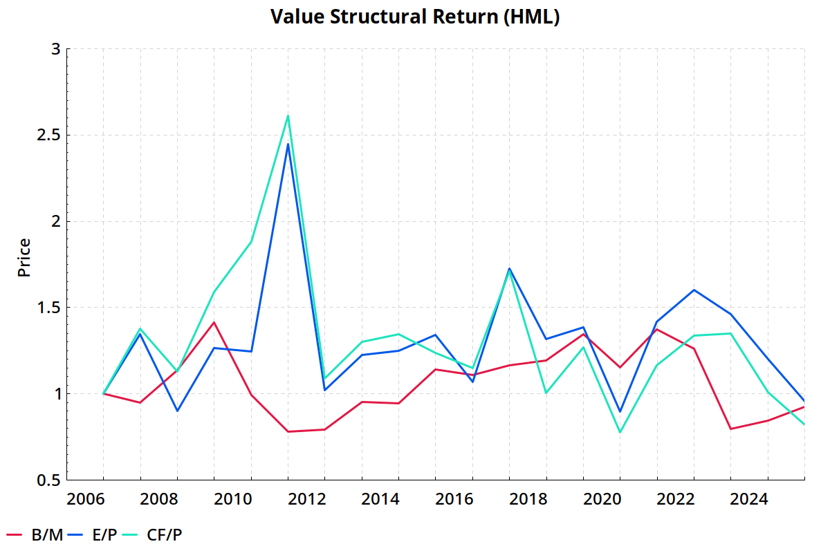
I also replicated the results using E/P and CF/P rather than B/M:
    --- E/P ---
    1963 to 2007:  5.4% return = -1.5% valuation + 7.0% structural
    2007 to 2020: -4.0% return = -0.8% valuation - 3.1% structural

    --- CF/P ---
    1963 to 2007:  4.8% return = -0.7% valuation + 5.5% structural
    2007 to 2020: -4.9% return = -0.5% valuation - 4.4% structural
Sensitivity to the choice of end date
The above results heavily depend on what end date you use because 2020 and 2021 were dramatic years for value, in opposite directions:
     B/M -- 2019 to 2020: -36.2% return = -20.7% valuation + -15.5% structural
     E/P -- 2019 to 2020: -27.5% return =  15.8% valuation + -43.3% structural
    CF/P -- 2019 to 2020: -30.9% return =  18.0% valuation + -48.9% structural

     B/M -- 2020 to 2021:  24.5% return =   7.0% valuation + 17.5% structural
     E/P -- 2020 to 2021:  20.3% return = -25.5% valuation + 45.8% structural
    CF/P -- 2020 to 2021:   9.6% return = -30.7% valuation + 40.3% structural
The negative valuation change is unfortunate for value investors, but not particularly worrying; valuation changes should even out over the long run. The decrease in structural return is more concerning because it could indicate a fundamental shift that makes value investing permanently less profitable.
That raises the question: How much does the structural return vary over time?
Over the full sample from 1927 to 2025, the value factor and its two components had the following annual standard deviations:
    total return:      16.2%
    valuation change:  24.7%
    structural return: 24.8%
The structural return varies quite a lot—more than the value factor itself.6
The difference in structural return between 1927–2006 and 2007–2025 was highly insignificant (t-stat = 0.496, p = 0.62). The standard error over a 19-year period (like 2007–2025) is 5.7%, so seeing the structural return drop to near zero isn’t that unlikely just by random chance.
But weak statistical evidence of a decline doesn’t mean there was no decline. Perhaps I’m being overly paranoid, but I want to dig deeper and see what it might mean if the structural return really did go down.
The next question I want to ask is, has the structural return ever been this low before?
Figure 1 shows the average structural return for rolling 15-year periods:
.png)
The next chart shows structural drawdowns for the value factor. Conceptually, a structural drawdown is a period where the value factor would’ve underperformed if the value spread had remained constant.
.png)
The current period is the 2nd worst in the historical sample, but not the worst: the value factor had a structural drawdown of nearly 70% from 1942 to 1946, and it did not fully recover until 1973. That’s a little reassuring—this sort of thing has happened before.
The next chart shows structural drawdowns alongside drawdowns for the valuation component and the value factor itself:
.png)
The weak structural return of the 2010s differs from the 1940s drawdown in that it coincided with an expansion of the value spread, which caused the value factor to experience its worst performance in recorded history.
What's happened since 2020?
Pease (2019)3 and Arnott et al. (2021)4 included data only up to 2019–2020. Since then, the value factor has experienced a minor resurgence. According to my replication:
2020 to 2025: 4.1% return = 8.5% valuation - 4.4% structural
This resurgence was accompanied by a negative structural return.
However, the structural return has enough variability that it’s hard to infer anything from five years of history:
These additional five years have provided (very) weak evidence for the hypothesis that value’s structural return is permanently dampened. But even with an additional five years of poor structural return, the decline is not statistically significant, nor has the structural return been as bad as it was in the 1940s era.
Elements of structural return
Can we say anything about why the structural return might have declined, assuming it wasn’t just random variation?
Let’s further decompose structural return into three components: growth + income + migration.
- Growth is the underlying growth in a company’s fundamentals.
- Income is the amount of dividends that a company pays out to shareholders.
- Migration is the conversion of value stocks into growth stocks, and growth stocks into value stocks. When a value stock’s price goes up and sufficiently outpaces its fundamentals, it migrates from the “value” bucket to the “growth” bucket (or to the “neutral” bucket in the middle). When that happens, value investors make money.
The growth component of return is almost always negative: in aggregate, growth stocks have stronger fundamentals growth than value stocks. That’s to be expected: the reason for a stock to have a high P/F ratio is that the market expects its F to go up.
Arnott et al. (2021)4 broke down structural return into its components, but did not offer much commentary. However, another article did: John Pease’s Risk and Premium: A Tale of Value (2019).
Pease presented this chart for the components of the value factor before and after 2006:
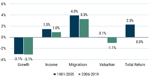
Source: Exhibit 27 in Pease (2019). Arnott et al. (2021) provides a similar decomposition in its Table 3, but combines growth + income into “income yield”.8
Pease went into detail about what explains each component. I can’t do justice to the full explanations, but in short:
- The growth component is unchanged. That suggests that there are no economic forces making value companies perform worse than they used to.
- Income has decreased because the market overall has gotten more expensive.
Illustrative example
Suppose value stocks pay a 6% dividend yield and growth stocks pay 4.5%. If the market goes up 50% while dividends don’t change, now value stocks yield 4% and growth stocks yield 3%. Even though growth and value stocks both went up by the same amount (50%), the income advantage for value stocks has been cut down from 1.5% to 1%.
- Migration return has declined. This component is the hardest to interpret.
The decline in migration return is the big question mark. Why did that happen? And will it persist?
Going deeper on migration
Migration occurs when the market re-evaluates its rating of a stock and changes the price, causing it to move from value to growth or vice versa. The most obvious reason for a re-rating is a fundamentals surprise: a company’s realized fundamentals growth outperforms or underperforms expectations.9
If migration declines, there are two possible explanations related to fundamentals surprises:
- Fundamentals surprises become smaller on average.
- Stock prices react less to fundamentals surprises.
(In mathematical terms: Migration occurs when a stock’s P/F ratio increases. Typically, this happens because F unexpectedly increases, and P subsequently increases by more than F. If migration does not occur, then either (1) F didn’t unexpectedly increase, or (2) P didn’t react as much to the change in F.)
If surprises get smaller, that’s bad for value. It means that a driving force behind the value factor has weakened.
The second explanation could be good or bad for value for complicated reasons. But before getting into that, let’s start by ruling out explanation #1.
Have fundamentals surprises shrunk?
Is (Systematic) Value Investing Dead?2 by Israel et al. (2021) analyzed, among other things, how well a stock’s valuation predicts its future fundamentals growth.
The relevant bit for our purposes comes from the paper’s Exhibit 9, column 8, which I used to derive the R2 between a stock’s price-to-fundamental ratio (P/F) and its subsequent one-year change in fundamentals (ΔF)10 for each year from 1987 to 2020.
Figure 5 answers the question: for each year, how well does a stock’s current P/F predict its ΔF?
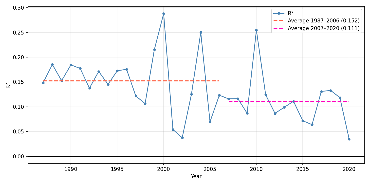
Why do we need to know R2 rather than slope?
The slope tells us how much a change in P/F predicts change in ΔF, but that number isn’t what we want. What we want to know is how much of the variance in ΔF is explained by P/F, which is to say we want R2.
For example, if the market’s discount rate decreases, then the value of distant cash flows goes up, and therefore the spread in P/F between stocks goes up. This causes the regression slope to flatten, even though the predictability of fundamentals growth did not change.
Israel et al. (2021)2 did not directly report R2, but I derived it by first reverse-engineering each year’s N from Exhibit 7, and then calculating R2 from N plus the slope and t-stat from Exhibit 9. For details, see Exhibit9.py.
Companies with low P/F (that is, value companies) tend to have low future fundamentals growth. When a stock has strong fundamentals but a low price, that’s Mr. Market saying “I don’t think these fundamentals are going to stay strong for much longer.”
Value investing has worked historically because the market’s predictions were overconfident: the cheap companies weren’t quite so bad as their prices implied. But the market was still directionally correct: in every year, companies with higher P/F had better fundamentals growth.
The question we want to ask is: did the migration return decline because fundamentals surprises shrank?
If surprises shrank, then R2 should have increased, but it didn’t. 1987–2006 had an average R2 of 0.152, and 2007–2020 had an average of 0.111. If anything, P/F got worse at predicting fundamentals growth (t-stat = 2.10, p = 0.04).
Keep in mind that Israel et al. (2021)2, Pease (2019)3, and Arnott et al. (2021)4 each used a different method to measure company fundamentals, so the results are not directly comparable. But the results should be moderately-to-strongly correlated with each other. I don’t have the data necessary to reproduce this analysis using Arnott et al.’s measure of value, but I would be surprised if the results were qualitatively different.
The market’s reaction to surprises
If fundamentals surprises haven’t shrunk, then the market must have reacted less to surprises. That can happen for two reasons:
- The market irrationally ignores new information.
- The market rationally ignores short-term surprises because it has better information about long-term growth.
If the market fails to (fully) incorporate new information about fundamentals, then value stocks stay cheap even as their prospects improve, and vice versa for growth stocks. In that case, the growth yield—the difference in fundamentals growth between value and growth stocks—should increase. (Recall that the growth yield is negative, so “increase” means “go toward zero”.)
But the growth yield did not increase post-2007. Pease (2019)3 found that it stayed exactly the same (to within 0.1 percentage points), and Arnott et al. (2021)4 found that it (slightly) decreased.
Under the hypothesis that the market irrationally ignores new information, I don’t know how much we’d expect the growth yield to increase, so I don’t know how to calculate the statistical significance of the empirical results. I suspect the significance is weak. Regardless, this provides non-zero evidence in favor of the second hypothesis: that the market is rationally ignoring surprises because it can see further ahead.
This makes some intuitive sense. Historically, companies’ fundamentals growth barely persisted: companies that had strong growth for a year were not detectably more likely to have strong growth for a second year (Chan et al. (2003)11; Chingono & Obenshain (2022)12). That implies that a fundamentals surprise shouldn’t much matter for future expectations. If the market persistently over-reacts to new information (a la De Bondt & Thaler (1985)13), then stocks will bounce between the value and growth buckets as the market repeatedly re-rates them—and value investors make money on every bounce. If the market stops over-reacting, then value investors lose access to this source of returns.
Arnott et al.’s statistical argument
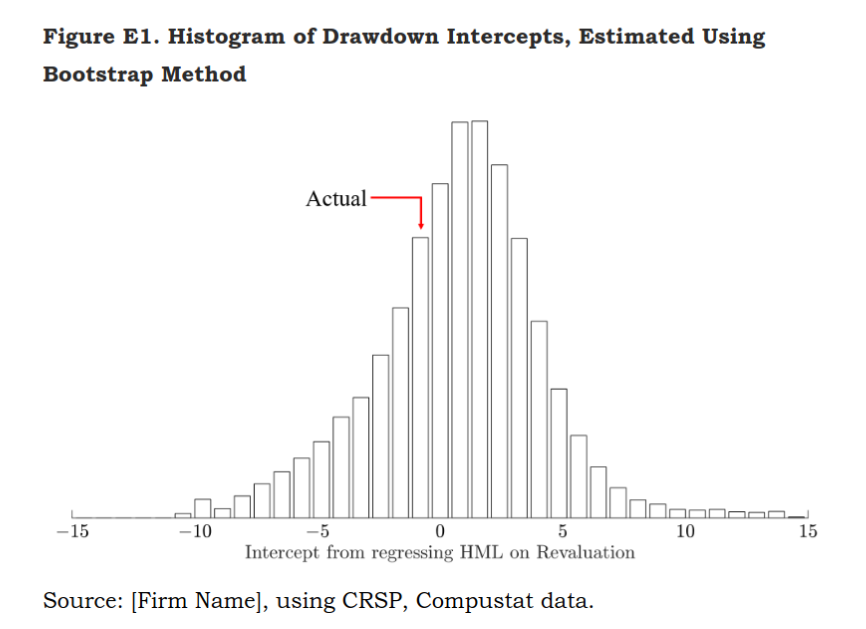
Before, I noted that the reduced structural return is statistically weak, with a t-stat of only 0.496. Arnott et al. (2021)4 raises a similar point about statistical reliability. In Appendix E, they note notes that the apparent weak structural return could be explained as selection bias from specifically looking at a period where value performed poorly. (If value had performed well, we wouldn’t be scrutinizing it like this.) The authors write:
When we explicitly analyze drawdowns, we introduce a selection bias by picking the sample to analyze based on the values of the dependent variable. In this case, we are studying the most recent 13½-year period precisely because of the poor performance of value, which is likely in part due to negative residuals.14 As an analogy, suppose that we were to analyze the performance of Tiger Woods from 1999 through 2004 (when he was the top-ranked player in the world for 264 consecutive weeks) but instead of looking at his total record, we only include the tournaments in which he played the worst. The resulting selection bias would lead us to struggle to explain why Tiger’s performance was not commensurate with his skill (alpha). Similarly, if we try to explain any factor’s performance, but only study a sample in which the factor performs poorly, we cannot hope to recover the factor’s true unconditional alpha; oversampling of negative residuals hopelessly contaminates the sample.
Although this mechanism is intuitive, an important question remains: Is the intercept [structural return] of -0.8% in the post-2007 period evidence of exceptionally improbable bad luck or just ordinary bad luck that we might expect to encounter when we examine any drawdown?
They found that the observed structural return was not statistically improbable:
Conclusion
To recap: In the post-2007 period, the structural return has averaged close to zero. This was not because fundamentals surprises happened less. The most plausible explanation is that it was just random variation—the difference in structural return pre- and post-2007 was highly non-significant (t-stat = 0.496).
The second most plausible explanation is that the market became more efficient at predicting long-term trends and started reacting less to year-by-year fundamentals surprises. If true, we should expect muted returns to the value factor going forward.
Appendix: Source code
- ValueAttribution.hs: Approximate structural return from Fama/French data.
- Exhibit9.py: Calculate R2 from Israel et al. (2020)2 data.
Changelog
- 2026-03-07: Add source code appendix; fix sign error on reported R2 values; fix sign error in a sentence (“worse” -> “better”).
Notes
-
The most rigorous value-skeptical article I’ve seen is Lev, B. I., & Srivastava, A. (2019). Explaining the Demise of Value Investing. ↩
-
Israel, R., Laursen, K., & Richardson, S. A. (2020). Is (Systematic) Value Investing Dead? ↩ ↩2 ↩3 ↩4 ↩5 ↩6
-
Pease, J. (2019). Risk and Premium: A Tale of Value. ↩ ↩2 ↩3 ↩4 ↩5
-
Arnott, R. D., Harvey, C. R., Kalesnik, V., & Linnainmaa, J. T. (2021). Reports of Value’s Death May Be Greatly Exaggerated. doi: 10.1080/0015198x.2020.1842704 ↩ ↩2 ↩3 ↩4 ↩5 ↩6 ↩7 ↩8 ↩9 ↩10 ↩11
-
Popular among non-value investors. ↩
-
I found that surprising. Intuitively, I’d expect the structural return to be fairly stable. I have no explanation for why the structural return fluctuates so much. ↩
-
I edited a label on the image to match my terminology. What I call “migration”, Pease called “rebalancing”. ↩
-
The numbers in Arnott et al. (2021) were much more dramatic, with a -13.2% income yield and 19.2% migration return pre-2007. That’s primarily because Arnott et al. defined the value factor as the cheapest 30% of companies minus the most expensive 30%, while Pease (2019) defined it as the cheapest 50% minus the total market. When the value and growth portfolios are more strongly differentiated, the difference in returns is larger.
I loosely replicated both studies’ pre-2007 results and found qualitatively similar results (with an Arnott-style construction producing much larger absolute values than Pease-style). I only looked pre-2007 because I don’t have individual stock data for the full later period. ↩
-
More generally, we could talk about “information surprises”: the market learns some new information and adjust prices accordingly. Information surprises are impossible to analyze in full generality—I can’t collect every conceivable source of information—so it’s easier to just focus on fundamentals surprises. But the principles I will discuss surrounding fundamentals surprises mostly also apply to other sorts of information. ↩
-
The paper defines “fundamentals” as current book value plus forecasted earnings for the next 24 months, where future earnings are discounted according to a stock-specific discount rate based on that stock’s beta. ↩
-
Chan, L. K. C., Karceski, J. J., & Lakonishok, J. (2003). The Level and Persistence of Growth Rates. doi: 10.1111/1540-6261.00540 ↩
-
Chingono, B. & Obenshain, G. (2022). Persistence of Growth. ↩
-
De Bondt, W. F. M., & Thaler, R. (1985). Does the Stock Market Overreact?. ↩
-
Footnote excerpted from Arnott et al.:
If we condition on the realization of the dependent variable as we do when we select periods based on value’s performance, we bias the estimated intercept. To see why, suppose that the model generating the data is \(y_i = a + b x_i + e_i\), where \(e_i\) is an innovation. Suppose further that \(a = 0\) and that the average \(e_i\) in our sample is zero. If we select observations in which \(y_i < 0\), it has to be that either \(b x_i < 0\) or \(e_i < 0\). That is, when we condition on the realization of \(y_i\), we indirectly condition on the realized value of the innovation, \(e_i\). We call this mechanism “oversampling bad luck”: the average \(e_i\) in the resulting sample is negative. If we take the observations in which \(y_i\) is negative and estimate a linear regression, the estimated intercept becomes negative; because the linear regression’s residuals add to zero, we push the average negative innovation into the intercept.