Should Patient Philanthropists Invest Differently?
TLDR: No.
Confidence: Somewhat likely.
Summary
Some philanthropists discount the future much less than normal people. For philanthropists with low discount rates, does this change how they invest their money? Can they do anything to take advantage of other investors’ high time discounting?
We can answer this question in two different ways.
Should low-discount philanthropists invest differently in theory? No. [More]
Should low-discount philanthropists invest differently in practice? The real world differs from the standard theoretical approach in a few ways. These differences suggest that low-discount philanthropists should favor risky and illiquid investments slightly more than high-discount investors do. But the difference is too small to matter in practice. [More]
Cross-posted to the Effective Altruism Forum.
Contents
- Summary
- Contents
- Background
- Theory
- Practice
- Conclusion
- Appendix A: Pedantry
- Appendix B: How I calculated historical optimal leverage
- Appendix C: How I calculated optimal private equity allocation
- Appendix D: Market volatility over longer holding periods
- Appendix E: Illiquidity in real estate
- Appendix F: Transformative changes to market behavior
- Notes
Background
Many people have a positive pure time preference: they prefer present consumption over future consumption, regardless of any empirical facts. Philanthropists shouldn’t have a pure positive discount rate, but they do have some legitimate reasons to discount the future, including:
- An extinction or economic collapse could render their money useless
- Their money could get expropriated (taxed, seized, or stolen)
- They might not be able to ensure that future generations continue spending their wealth in the ways they want
(Some people talk about impatient vs. patient philanthropists who have positive vs. zero pure time preference, or urgent vs. patient longtermists who believe we do vs. don’t live in a particularly important time. For this essay, I’m talking about low-discount vs. high-discount philanthropists. Urgent longtermists usually have high discount rates and patient longtermists usually have low rates, but it’s not a 1:1 correspondence.)
Many philanthropists don’t want to spend all their money at once; any money they don’t spend gets invested. And we would like to know how we should invest. For this essay, I will ask: how does optimal investment strategy change with discount rate? For philanthropists with unusually low discount rates, what should they do differently?
Suppose philanthropists have a pool of wealth that they invest, and they consume a fixed proportion of wealth each year. (For a philanthropist, donating to charity counts as consumption.) They get some utility every time they spend money. What investment strategy maximizes expected utility? And how does that investment strategy vary as a function of discount rate?
Theory
Merton (1969)12 derived a formula for how much leverage investors should use and how quickly they should spend down their assets (given some simplifying assumptions). Merton found that the optimal investment allocation does not depend on the investor’s discount rate.
In theory, the optimal allocation only depends on three things:
- assets’ expected returns
- assets’ covariances with each other
- the investor’s relative risk aversion (RRA)
The first two are properties of the assets themselves, not of the investors. The only factor that (theoretically) should cause two investors to behave differently is their degree of risk aversion.
The optimal rate of consumption3 does depend on one’s discount rate.4 But the discount rate does not affect the choice of investment.
Merton’s proof depends on four key assumptions:
- Investors have constant relative risk aversion.
- Asset prices follow log-normal distributions.
- Asset returns are independent across time.
- Assets can be traded continuously.
The assumption of constant relative risk aversion means that investors’ risk preferences do not change when their wealth increases or decreases. This might be false, but it’s close enough to true, so I won’t question this assumption for now.5
If asset prices don’t follow log-normal distributions, then you cannot fully describe assets’ performance in terms of mean and covariance. This affects investment strategy (mostly by making us more concerned about tail risk), but it doesn’t affect how quickly we should consume.
The third assumption—time independence—matters the most for our purposes. If investment returns tend to regress to the mean—in other words, if present and future returns are anticorrelated—then this changes how you should invest.
Why? If returns are anticorrelated, then if you lose some money now, that increases your expectation that you’ll make it back later. It also decreases the probability that you’ll be able to compound unusually high returns for multiple years in a row. This matters regardless of discount rate, but it matters more for investors with low discount rates because they care more about fluctuations in their future wealth.
The fourth assumption—perfect liquidity—does not directly relate to investors’ discount rates, but it can still matter, as I discuss below.
Practice
Low-discount philanthropists might invest differently for three reasons:
- long-term mean reversion
- subjective uncertainty about future returns
- illiquidity premium
Long-term mean reversion suggests that:
- Risk-averse (specifically, more risk-averse than logarithmic) low-discount investors should use more leverage than risk-averse high-discount investors.
- Risk-tolerant (more risk-tolerant than logarithmic) low-discount investors should use less leverage than risk-tolerant high-discount investors.
(Confidence: Highly likely.)
This crude drawing shows how leverage varies for low-discount vs. high-discount investors after accounting for long-term mean reversion:
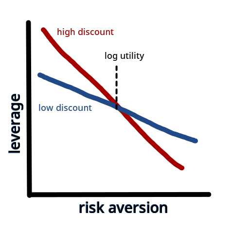
But this drawing overstates the size of the effect. (Or at least it would, if it had any labels or scale.) Empirically (based on historical returns), mean reversion only slightly changes the optimal amount of leverage, and probably doesn’t matter in practice. (Confidence: Likely.) [More]
Over longer time periods, investors have greater subjective uncertainty about how markets will behave. This creates subjective long-term momentum, which has the opposite effect of mean reversion. (Confidence: Likely.) And, like with mean reversion, this effect only slightly differs between low- and high-discount investors. (Confidence: Likely.) [More]
If long-term illiquid investments earn significantly higher returns, then investors with low discount rates prefer them relative to high-discount investors. (Confidence: Highly likely.) [More] But empirical data suggests they don’t earn an illiquidity premium, so illiquid investments don’t look particularly compelling, regardless of discount rate. (Confidence: Likely.) [More]
Some investors may prefer illiquid investments for behavioral reasons due to their (perceived but not actual) reduced volatility, and for these investors, a lower discount rate suggests a higher allocation to private equity. [More]
As a final point, conventional wisdom says long-term investors should take more risk. Conventional wisdom is correct, not because long-term investors have a lower discount rate, but because they can expect to earn future income which reduces their effective risk. So this observation is not relevant to how low-discount philanthropists should invest. (Confidence: Almost certain.) [More]
1. Long-term mean reversion
When Merton proved that asset allocation does not depend on time discounting, he assumed that investment returns are independent across time. But that’s not quite true. Historical evidence (weakly6) suggests that stocks exhibit long-term mean reversion. When prices go up a lot over a 3+ year period, they have a slight tendency to go back down. And when they go down over 3+ years, they have a similar tendency to rebound upward. That makes stocks a little less risky over longer holding periods.
How does this affect low-discount investors relative to high-discount investors?
Long-term mean reversion decreases the variance of an investment while keeping its geometric mean fixed, and decreasing the arithmetic mean.
Low-discount investors feel the decreased volatility more strongly than high-discount investors do because they care more about their investment performance in later years. But for the same reason, they more strongly feel the decrease in arithmetic mean return.
How this affects investors depends on their degree of risk aversion:
- For investors with logarithmic utility, maximizing utility is equivalent to maximizing geometric mean, so they don’t care at all about mean reversion.
- For “risk-averse” investors (those with sub-logarithmic utility), they care more about volatility than about arithmetic mean, so they like mean reversion.
- For “risk-tolerant” investors (those with super-logarithmic utility), they care more about arithmetic mean than about volatility, so they dislike mean reversion.
Risk-averse low-discount investors want more leverage than risk-averse high-discount investors, while risk-tolerant low-discount investors want less leverage than risk-tolerant high-discount investors.7
More precisely:
- At logarithmic utility, discount rate does not matter.
- For risk-averse investors, desired leverage decreases with discount rate.
- For risk-tolerant investors, desired leverage increases with discount rate.
At least that’s the hypothesis.
How strong are these effects? It turns out, pretty weak. I used data from The Rate of Return on Everything, 1870–20158 and the Ken French Data Library to calculate historical utility-maximizing leverage for an equity investor in three environments: the US market from 1872 to 2015; the UK market from 1871 to 2015; and the developed-world markets (excluding the US) from 1990 to 2021.
Each of these historical cases confirmed the hypothesis, but they showed a weak effect size.
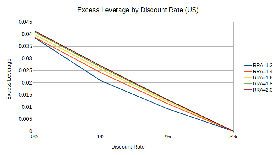
These two charts show excess leverage by discount rate for US and UK equities, compared to a baseline 3% discount rate:
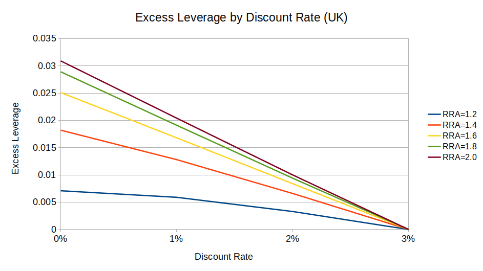
(I didn’t graph excess leverage for RRA < 1 because a solution usually does not exist.9)
We can see from these charts that a zero-discount investor wants at most 4 percentage points more leverage than an investor with a 3% discount rate (1.78:1 vs. 1.74:1, respectively10). And the effect gets smaller as relative risk aversion (RRA) gets closer to 1.
So, while long-term mean reversion does theoretically change how low-discount philanthropists should invest, the difference is effectively a rounding error. (I can’t even say whether philanthropists should prefer (say) 1.5:1 leverage or 2:1 leverage, much less 1.78:1 or 1.74:1.)
(I should mention that, while equities exhibit long-term mean reversion, bonds appear to show long-term momentum, which would produce the opposite effect. However, historically, bonds did not have stable geometric means, and the historically optimal leverage for bonds showed the same results as for equities with respect to discount rate and RRA. And as with equities, the effect is too small to matter in practice.)
See Appendix B for the details of my calculations.
2. Uncertainty about future returns
Pastor & Stambaugh (2012)11 showed that, due to uncertainty about average future returns, investors’ subjective volatility increases with time horizon. This produces the opposite effect of mean reversion: risk-averse low-discount investors want less leverage than risk-averse high-discount investors, while risk-tolerant low-discount investors want more leverage than risk-tolerant high-discount investors.
Behold, another crudely-drawn graph:
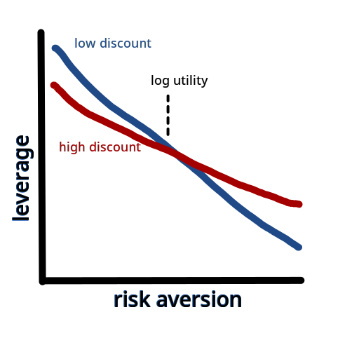
According to Pastor & Stambaugh, parameter uncertainty matters more than long-term mean reversion, but less than twice as much more. That means the combined impact of mean reversion + uncertainty has the opposite sign and a smaller magnitude than mean reversion alone. As we saw, the practical impact of mean reversion only varies slightly between low-discount and high-discount investors, so the impact of mean reversion + uncertainty varies even less.
Pastor & Stambaugh did not look at parameter uncertainty across discount rates, so I did my own analysis. I tested historically optimal leverage with parameter uncertainty by adding an “uncertainty factor” to the average return. This uncertainty factor was a normally-distributed random number between –2% and 2% (with that range representing the 95% confidence interval of the true average return).
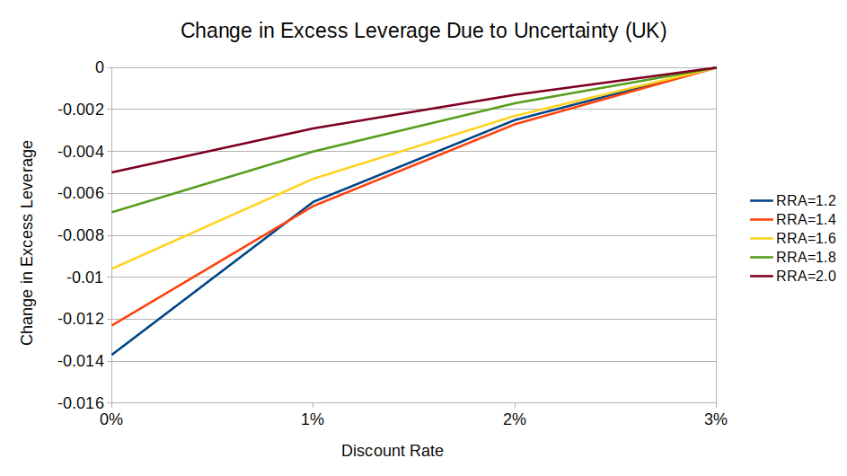
As expected, the uncertainty factor does not affect optimal leverage for logarithmic-utility investors. For risk-averse investors, uncertainty decreases optimal leverage, and it decreases more for low-discount investors than for high-discount ones:
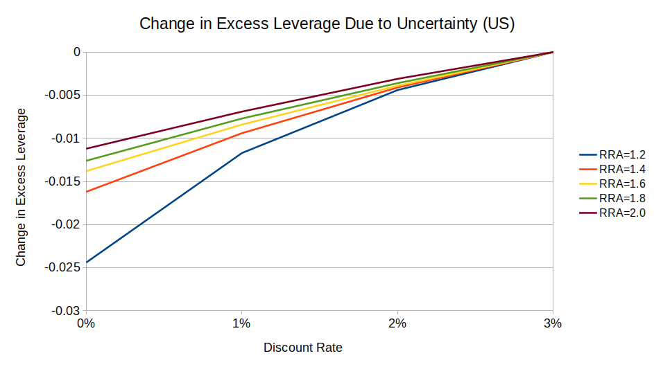
(UK equities show the same pattern, but a weaker effect.12)
When incorporating both mean reversion and uncertainty, risk-averse low-discount investors still preferred to use more leverage than risk-averse high-discount investors, but by a smaller margin than they would given certainty:13
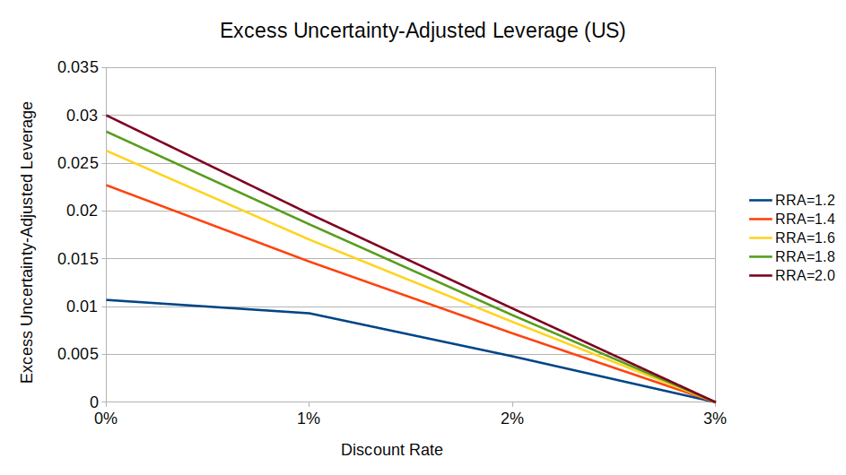
(Notice how on this chart, the maximum excess leverage is ~0.03, while in the original chart with fixed parameters (“Excess Leverage by Discount Rate (US)”), the max was ~0.04.)
UN equities show a similar effect, except that in some cases, low-discount investors want (slightly) less leverage than high-discount investors:
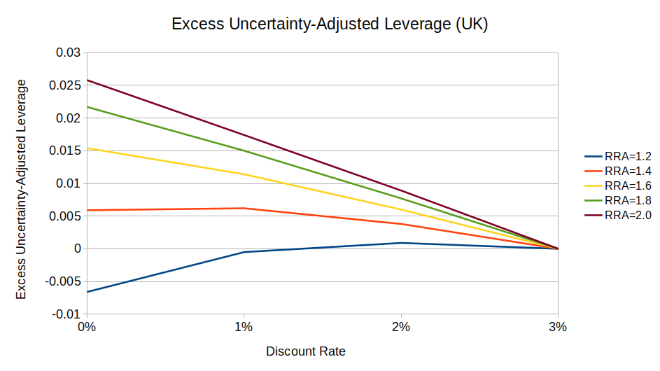
For risk-tolerant investors (with super-logarithmic utility), adding uncertainty increases desired leverage, and the effect is larger for low-discount investors. However, it’s hard to quantify this effect because at low discount rates, sufficiently risk-tolerant investors want to use infinite leverage. (I would interpret this as evidence that philanthropists don’t have larger-than-logarithmic utility functions.)
Note that Pastor & Stambaugh found that parameter uncertainty outweighed mean reversion, while I found the opposite. If my analysis had looked more like Pastor & Stambaugh’s, then we would get the opposite result after accounting for both mean reversion and parameter uncertainty. But it doesn’t really matter because the effect is small either way.
3. Illiquidity premium
Low-discount philanthropists might not need to spend their money for a long time. Does that mean they should buy illiquid investments?
I will focus on private equity because it’s the most straightforward type of illiquid investment, and it has a clear analogue in public equity. First I will consider what illiquidity premium we should expect in theory for private equity. Then I will look at the observed illiquidity premium, and then attempt to reconcile the two.
See Appendix E for some discussion of illiquidity in real estate.
Theoretical illiquidity premium
In theory, should low-discount investors like illiquid investments more than high-discount investors do?
People’s preferences for liquidity do not directly depend on discount rate, but they do depend on their consumption rate. If you want to spend a (relatively) large percentage of your capital each year, then you’re more reluctant to lock up a big chunk of money in illiquid investments. There’s a risk that the market tanks and you end up spending down too big a proportion of your liquid assets.
All else equal, a higher discount rate means a higher spending rate. Low-discount philanthropists may consume only a tiny fraction of their wealth each year, which means they’re not concerned about over-spending their liquid investments.
In a two-asset model with public equity and (synthetic) private equity, low-discount investors allocate 1 to 5 percentage points more to private equity than high-discount investors:
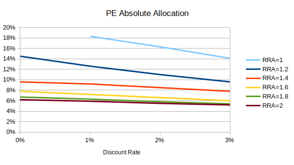
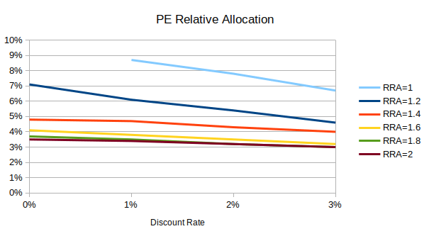
(“Absolute” is the allocation as a percentage of wealth/liquidation value; “relative” is the allocation as a percentage of public + private allocation. Public + private absolute allocation can exceed 100% due to leverage.)
See Appendix C for the details on methodology.
Observed illiquidity premium
How large a premium can investors earn by holding private equity instead of public stocks?
Historically, private equity in the United States earned a 3% premium (Harris et al., 201414; Kaplan & Sensoy, 201515). However, this premium is not explained by illiquidity. The private equity premium is fully subsumed by a leveraged small value portfolio in public equities (Chingono & Rasmussen, 201516; Ilmanen et al., 201917; Stafford, 201718). In fact, private equity has (large but statistically insignificant) negative alpha compared to leveraged small value.
Given zero (or negative) alpha for private equity, investors do not want to hold it, regardless of discount rate.
Reconciling predicted and observed illiquidity premiums
If theory predicts an illiquidity premium, why don’t we see one in historical data?
The most common explanation (e.g., as given in Ilmanen et al., 201917 and Chingono & Rasmussen, 201516) is that investors are willing to pay a premium for the return smoothing provided by private equity. Unlike a public market where the price updates many times per second, private equity firms have leeway to report essentially whatever valuations they want. They tend to under-report drawdowns, making returns for private companies look more consistent than their public counterparts, but with no corresponding decrease in true underlying risk (Welch & Stubben, 201819). (In 2022 when the S&P 500 experienced a 20+% drawdown, the average private equity firm reported a 0% change in valuation, which is absurd on its face, but they’re allowed to do it.)

Investors’ preference for return smoothing is, in some sense, irrational—it doesn’t provide any financial benefit. But if you know that seeing your portfolio lose value will give you anguish, and might cause you to make a bad decision, then it could be rational to tie yourself to the mast by buying private equity.
Evidence suggests that, at least in the current market environment, rational investors should not invest in private equity, regardless of discount rate. But human investors with typical human flaws may do better by investing in private equity, even if it’s not technically optimal. And low-discount investors should allocate on the order of 5 percentage points more to private equity than high-discount investors do. Sophisticated institutional investors tend to allocate 10% to 15% to private equity,20 which would suggest a 15% to 20% allocation for philanthropists with low discount rates. This is a small enough difference that it might not matter in practice, but it’s still a much bigger difference than we found for long-term mean reversion or parameter uncertainty.
I personally do not invest in private equity because I’m not concerned about the behavioral issues (and because it’s hard to invest in, but that’s secondary).
A note on conventional wisdom
Conventional wisdom says that investors with long time horizons should take on more risk. Why? Does that apply to low-discount philanthropists?
The conventional wisdom is correct for most people, but not because long-term investors inherently want more risk. Rather, long-term investors (usually) expect to earn more income in the future, and they should count that income as part of their investment portfolio. After factoring in their future income, they should seek the same amount of risk as a short-term investor.
For example, say Alice is retired with $1 million, and she invests her retirement fund in 50% stocks, 50% bonds. Bob has $100,000 in savings and expects to earn another $900,000 before he retires. He invests 100% of his savings into stocks. Bob’s portfolio looks riskier than Alice, but it’s actually less risky: Alice has 50% of her portfolio in stocks, while Bob effectively only has 10% after accounting for his future income. In theory, If Bob used 5:1 leverage, he would get his effective stock allocation up to 50%, although that’s probably not feasible in practice.
For low-discount philanthropists, how much risk to take depends on what money they expect to earn in the future. That depends on their personal income plus the income of all likeminded philanthropists plus the wealth and income of any people in the future who will become likeminded. Figuring out all those details is beyond the scope of this essay. The bottom line is: yes, the conventional wisdom is correct in a sense, but it doesn’t contradict my earlier claim that an investor’s risk appetite does not depend on time horizon, and it doesn’t have anything to do with discount rates.
Conclusion
In summary:
- According to standard theory, investors should not change their asset allocation based on their discount rate.
- Standard theory assumes that time periods are independent and that all investments are highly liquid, both of which are (sometimes) false.
- Investment returns are not entirely independent over time. This has a nonzero but negligible effect on high- vs. low-discount investors.
- It looks like illiquid assets don’t earn a significant premium, so low-discount investors shouldn’t prefer them.
Therefore, low-discount philanthropists don’t need to allocate any differently than high-discount investors.
Appendix A: Pedantry
In this essay, I somewhat conflated low-discount philanthropists with long-term philanthropists, but they’re not necessarily the same thing. For our purposes, “long-term” means you have a (relatively) long time horizon. A 3% discount rate would be considered high, but a philanthropist with a 3% discount rate could still easily have a 50+ year time horizon.
A low discount rate is not the same thing as longtermism (at least the way I use the term). A longtermist might have a high discount rate, for instance if they believe extinction is likely to render their funds useless in the near future, or if they expect not to be able to preserve the intent of their endowment across multiple generations. And someone with a 0% discount rate doesn’t have to be a longtermist—e.g., some form of person-affecting view could preclude longtermism even with no time discounting.
Philanthropists with particularly pessimistic beliefs about existential risk might have higher discount rates than normal people, which would suggest doing the opposite of what low-discount philanthropists do (which, if I’m right, is nothing, so it doesn’t matter either way).
Not all low-discount investors are low-discount philanthropists, but I use the terms interchangeably because I only care about investors who are also philanthropists.
Appendix B: How I calculated historical optimal leverage
I used data from The Rate of Return on Everything, 1870–2015 (RORE)8 and the Ken French Data Library, focusing on four data series:
- US equities 1926 to 2021, from Ken French
- Developed ex-US equities 1990 to 2021, from Ken French
- UK equities 1899 to 2015, from RORE
- US equities 1872 to 2015, from RORE
(In the main essay, I did not discuss #1 because it’s mostly a subset of #4. I only looked at both as a sanity check.)
I implemented the standard Ramsey model of intergenerational welfare where we have a pool of wealth that we invest at some rate of return, and every year we consume some fixed percentage of our wealth. We have a utility function over consumption, and total utility is the sum of discounted utility of consumption for each period. Then we simultaneously solve for the optimal amount of portfolio leverage and optimal rate of consumption. (For this essay, we don’t care about consumption, but we still have to solve for both variables.)
Applying this model over historical data requires making some modifications. We can’t calculate total utility out to infinity because we only have a finite sample of real historical financial returns. Naively, we could simply maximize utility over the sample we have, but this has two major problems:
- We don’t discount the last year all that much relative to the first year. Any money left over at the end has a high opportunity cost. The optimizer wants to end up with as close to $0 as possible, so it recommends consuming at a faster rate than we’d want to if we had an infinite time horizon.
- The outcome strongly depends on what happens to our investments near the beginning of the sample because the beginning is discounted the least.21
I implemented (somewhat ad-hoc) solutions for both of these problems:
- Loop through the historical sample multiple times, extending it until it repeats for 1000 years.22 The 1000th year has minimal impact on total utility, so the optimal solution over 1000 years looks almost exactly like the optimal solution over infinity years.
- Instead of only starting at the first year in the sample, calculate total utility for every possible starting year and then take the average.
Tables of results
The tables below give optimal leverage and consumption for various rates of relative risk aversion and discount rates, given a fixed-point expected return (no parameter uncertainty). I included 1% and 3% discount rates except for at 0.75 RRA, in which case the solution did not always exist, so I included higher discount rates instead. For RRA > 1, I also included a 0% discount rate.
For Ken French data (Tables 1 and 2), I applied discounting and consumption on a monthly basis and estimated the cost of leverage at the risk-free rate as given in the data.
For RORE data (Table 3), I applied discounting and consumption on an annual basis and estimated the cost of leverage at 0% because I don’t have data on the risk-free rate going back far enough. This is wrong, but it doesn’t matter for our purposes.
Table 1. US equities, 1926 to 2021.
| RRA | Discount | Leverage | Consumption |
|---|---|---|---|
| 0.75 | 1% | DNE | DNE |
| 0.75 | 3% | 2.20 | 0.43% |
| 0.75 | 5% | 2.36 | 2.65% |
| 1 | 1% | 2.16 | 1.00% |
| 1 | 3% | 2.16 | 3.02% |
| 2 | 0% | 1.47 | 5.56% |
| 2 | 1% | 1.45 | 6.00% |
| 2 | 3% | 1.40 | 6.89% |
Geometric mean is maximized at 1.90 leverage.
Table 2. Developed ex-US equities, 1990 to 2021.
| RRA | Discount | Leverage | Consumption |
|---|---|---|---|
| 0.75 | 1% | DNE | DNE |
| 0.75 | 3% | 1.57 | 2.09% |
| 0.75 | 5% | 1.58 | 4.84% |
| 1 | 1% | 1.56 | 1.05% |
| 1 | 3% | 1.55 | 3.03% |
| 2 | 0% | 1.48 | 2.98% |
| 2 | 1% | 1.45 | 3.43% |
| 2 | 3% | 1.42 | 4.44% |
Geometric mean is maximized at 1.17 leverage.
Table 3. UK equities, 1871 to 2015.
| RRA | Discount | Leverage | Consumption |
|---|---|---|---|
| 0.9 | 3% | 1.92 | 1.92% |
| 0.9 | 5% | 1.88 | 4.10% |
| 1 | 1% | 1.86 | 1.00% |
| 1 | 3% | 1.86 | 2.98% |
| 2 | 0% | 1.79 | 5.36% |
| 2 | 1% | 1.78 | 5.69% |
| 2 | 3% | 1.76 | 6.54% |
A portfolio that combines the US market beta + value + momentum factors shows the same pattern (with RRA < 1, optimal leverage increases with discount rate; with RRA > 1, optimal leverage decreases with discount rate). I calculated this portfolio using Ken French data as the simple sum of ‘Mkt’ + ‘HML’ + ‘Mom’ (UMD).
Table 4. US market beta + value + momentum factors, 1927 to 2021.
| RRA | Discount | Lev | Consumption |
|---|---|---|---|
| 0.9 | 3% | 3.05 | 0.14% |
| 0.9 | 5% | 3.15 | 1.53% |
| 1 | 1% | 3.04 | 1.00% |
| 1 | 3% | 3.04 | 3.04% |
| 2 | 0% | 1.57 | 9.59% |
| 2 | 1% | 1.56 | 9.92% |
| 2 | 3% | 1.55 | 10.82% |
This chart shows excess optimal leverage (relative to a baseline 3% discount rate) for a US market + value + momentum factor portfolio with RRA > 1:
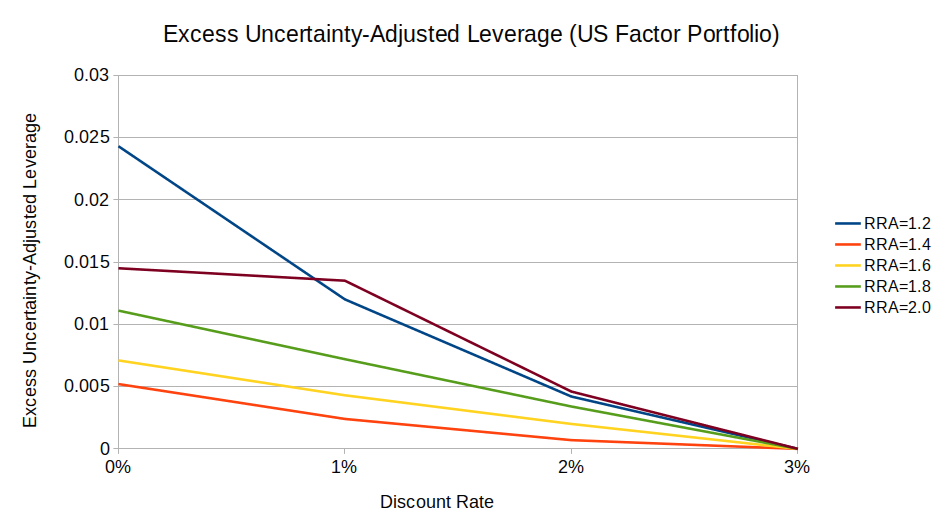
This suggests that, for a factor investor, discount rate matters somewhat less than for a passive investor.
Appendix C: How I calculated optimal private equity allocation
There is some pre-existing literature on the theoretical illiquidity premium, such as Ang (2014).23 However, I could not find any research on how the illiquidity premium varies as a function of discount rate, so I did my own analysis.
I calculated the optimal allocation across two assets labeled “public equity” and “private equity”. I used RORE8 data on the US stock market back to 1872 as the public equity component. For private equity, we don’t have data going back very far, so as a proxy, I used RORE data on UK public equities. Private equity behaves mostly like private equity, but not exactly; similarly, UK equity behaves mostly like US equity, but not exactly, so for this test, I took historical returns for UK public equity and pretended they represented private equity. Then I multiplied the UK annual returns by 1.5 to account for the fact that private equity tends to be more volatile.
The resulting “private equity” return series has an 11.6% annualized return, compared to 8.9% for US public equity; this matches the observed 3% private equity premium.
In my simulation, investors can only allocate to private equity once every 10 years. Any money they invest stays locked up, and they can rebalance at the end of every 10-year period. Investors can use leverage on public equity but not on private equity.24
This produced the following relative allocations to private equity at various discount rates and levels of risk aversion:

“Private equity” had +6.6% alpha over public equity. If we subtract 6.6% from private equity returns to give it zero alpha, the optimal allocation becomes 0% regardless of risk aversion or discount rate.
If we add a pure +2% premium to private equity, this increases the optimal allocation, and also increases the differential between low- and high-discount investors, with low-discount investors now allocating 2 to 9 percentage points more to private equity than high-discount investors:
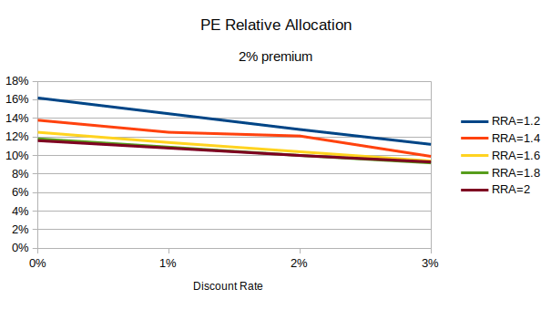
If we make the lockup period longer than 10 years, it reduces the optimal allocation for all investors, and it increases the differential between low- and high-discount investors. The opposite happens if we shorten the lockup period.
In some cases, there is no optimal allocation because it’s always better to delay spending indefinitely. This condition holds at (RRA = 1, discount rate = 0%) and at RRA < 1 for sufficiently low discount rates (including RRA = 0.8, discount rate = 3%).
(Originally, I wanted to set the average return of the “private equity” asset such that the high-discount-optimal allocation reflects the real-world allocation to private equity, and then calculate the low-discount-optimal allocation given the same inputs. But I couldn’t find good data on the total market cap of private equity, so I just used inputs that seemed reasonable.25)
Appendix D: Market volatility over longer holding periods
Stock markets exhibit long-term mean reversion. As shown in Appendix B, this encourages risk-averse investors with lower discount rates to use more leverage. I calculated this using some complicated26 and hard-to-intuit math. For a more intuitive approach, we could look at market volatility over different holding periods.
Jeremy Siegel’s Stocks for the Long Run27 looked at the US equity market from 1802 to 2012 and found that volatility decreases over longer holding periods. I extended these results to global equities using data from The Rate of Return on Everything, 1870–20158. I looked at the annualized standard deviation28 of stock markets in 8 different countries29 for holding periods ranging from 1 to 30 years.30
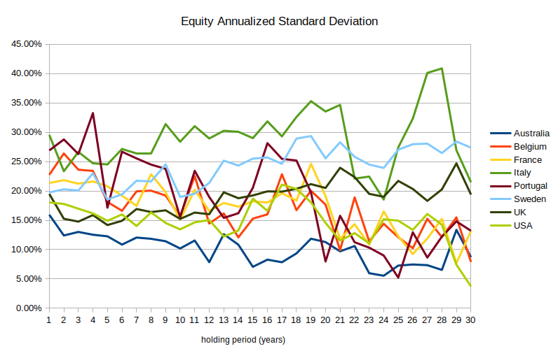
(30 years is more or less the longest holding period we can say anything about because there are only four non-overlapping 30-year periods in the sample.)
This chart shows a weak downward trend. On average, for every year that you increase the holding period, the annualized standard deviation decreases by 0.14% (p < 0.002, but you shouldn’t take this p-value literally31), although this number is pretty sensitive to how far you extend the regression—if you exclude the particularly-noisy 21 to 30 year holding period range, the slope reduces to 0.004% with p = 0.94. And we can’t tell if the trend extends beyond 30 years, but it doesn’t look like it does.32 So stocks are somewhere between 0 and 4 percentage points less volatile over 30 years than over 1 year.
(Siegel (2014)27 found a larger and more unequivocal mean reversion effect. That’s mostly because it only covered the US market, and you will notice that in the table above, the United States shows stronger mean reversion than most countries.)
At the same time, stock markets’ arithmetic means decrease over longer holding periods:
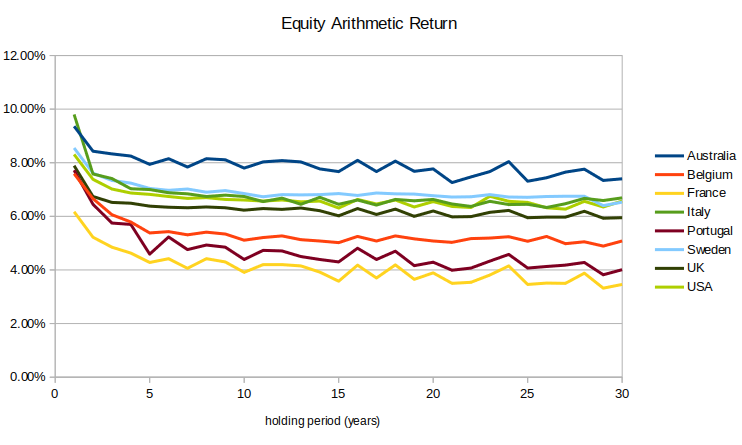
Long-term mean reversion works in favor of risk-averse investors (RRA > 1) and against risk-tolerant investors (RRA < 1).
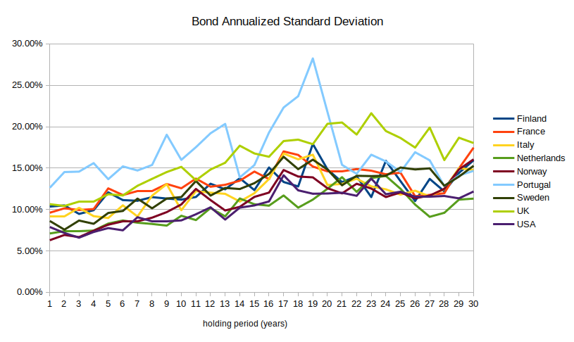
Bonds get more volatile as you increase the holding period, from an average of 7% annualized volatility up to 12%:33
Appendix E: Illiquidity in real estate
Real estate is less liquid than stocks, but not in a way that benefits low-discount philanthropists. Real estate costs money to trade, but it doesn’t have lockup periods like private equity, so we shouldn’t expect to see an illiquidity premium. There might be a “trading cost premium”, which benefits investors with long holding periods, but real estate investors tend to have long holding periods anyway, so this doesn’t make real estate look particularly good from a low-discount perspective.
The main bottleneck to real estate investing is not liquidity but diversification. To properly diversify your real estate portfolio, you’d need to spend tens of millions of dollars buying dozens of properties. If you do have that much money, then investing in real estate is probably smart. Indeed, many wealthy, long-term-oriented investors such as university endowments own a lot of land.
Illiquidity premium in 100-year leases
Could low-discount philanthropists do well by buying much longer-term illiquid investments, such as 100-year property leases? Phil Trammell proposed doing this. He claims that if you buy a house and simultaneously sell a 100-year lease, you gain the right to use the land 100 years from now and you only have to pay 10% of its present value. (I couldn’t find good data on the cost of a 100-year lease, so I’ll take his word for it.)
A 10% price implies a 2.3% interest rate (\(1.023^{100} = 10\)), which sounds basically fair—maybe even too low. As an illustration, suppose you have $1 million and you’re deciding between two choices:
- Buy 10 houses for a total of $10 million and simultaneously sell a 100-year lease on each of them. You spend $1 million on net, and you get 10 houses 100 years from now.
- Buy one house for $1 million and rent it out. Suppose the annual rent is 2.3% of the value of the house. Then in 100 years, you use the earned rent to buy the other nine houses. You spend $1 million, and you get 10 houses 100 years from now.
These two scenarios cost the same and provide the same value. And 2.3% is on the low end of rental yields; if you can earn a higher yield than that, it would make more sense to simply buy a house rather than buy 10 houses and sell 100-year leases on them.
(Why doesn’t the market set a higher implied interest rate on 100-year leases? Probably because houses are tradeable(ish): your money isn’t truly locked up for 100 years because you can sell the house at any time. So in an efficient market, the implied interest rate should equal the expected market yield (plus some other factors like differential taxes, maintenance costs, cost of selling the house multiplied by probability of wanting to sell, etc.)
Appendix F: Transformative changes to market behavior
Over sufficiently long time horizons, markets might see significant changes to investment performance, such as:
- Technological growth compounds on itself (possibly due to transformative AI), causing the rate of exponential growth to accelerate, greatly increasing returns.
- We reach the physical limits of economic growth, and investments stop growing exponentially.
There might be interesting things to say about these or other possible futures that break the current paradigm of consistent exponential growth. But that’s much more speculative, and I consider it out of scope for this essay.
If you expect the economy to radically change in (say) 1000 years, but not to change much before then, then that doesn’t significantly affect how to invest today.
If you expect (with non-trivial probability) major changes in the near future (such as due to transformative AI), that does change how you should invest, but I’m not sure how,34 and that’s a question for another time.
Notes
-
Robert Merton (1969). Lifetime Portfolio Selection Under Uncertainty: The Continuous-Time_case. Read status: Multiple full read-throughs. This is a seminal paper so I’m highly confident that it’s good. ↩
-
Not all of the results I describe are original to Merton, but he provided the first single paper that proves all of them. ↩
-
For our purposes, “consumption” refers to anything we do with money other than re-investing it. For example, if we donate money, that counts as a form of consumption. ↩
-
The exact solution for the optimal consumption rate is given in formula (42) of Merton (1969). All else equal, the rate of consumption increases linearly with the discount rate. ↩
-
If you become more risk-averse as you get wealthier, then you should consume a larger proportion of wealth when you’re wealthier, and vice versa. ↩
-
Paul McCaffrey (2022). Equity Risk Premium Forum: Term Structure, Mean Reversion, and CAPE Reconsidered. Partial transcript of a discussion between Laurence B. Siegel, Rob Arnott, Elroy Dimson, William N. Goetzmann, Roger G. Ibbotson, Antti Ilmanen, Martin Leibowitz, Rajnish Mehra, and Jeremy Siegel.
Some relevant quotes:
Goetzmann: “The evidence is always a bit marginal and depends on your assumptions and on where you get the data.”
Ilmanen: “I see evidence of mean reversion over time horizons from 3 years up to 15 years. […] The evidence is really fuzzy, and usable or actionable evidence is almost zilch because of all this horizon uncertainty.” ↩
-
One thing I learned from writing this essay: I find it easy to think about two-dimensional relationships (“how does Y change as a function of X?”), but far harder to think about three-dimensional relationships (“how does ‘how does Z change as a function of Y’ change as a function of X?”). I kept finding myself getting the variables mixed up. ↩
-
Òscar Jordà, Katharina Knoll, Dmitry Kuvshinov, Moritz Schularick & Alan M Taylor (2019). The Rate of Return on Everything, 1870–2015. ↩ ↩2 ↩3 ↩4
-
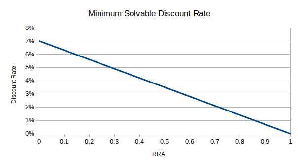
To be precise, if prices follow a log-normal distribution, then a solution exists only when the following condition holds, where \(\delta\) is the discount rate, \(\gamma\) is the rate of relative risk aversion, \(\mu\) is the expected (geometric) portfolio return minus the risk-free rate, and \(\sigma\) is the portfolio standard deviation:
\[\frac{-\delta}{\gamma} + (\mu + \sigma^2/2)\frac{1-\gamma}{\gamma} - (1 - \gamma)\sigma^2/2 < 0\](Formula taken from Levhari & Srinivasan (1969). “Optimal Savings Under Uncertainty.”)
This graph shows the minimum solvable discount rate as a function of RRA for \(\mu = 7\%, \sigma=18\%\):
-
These specific numbers come from US equities with risk aversion coefficient = 2. ↩
-
Lubos Pastor & Robert F. Stambaugh (2012). Are Stocks Really Less Volatile in the Long Run? Read status: I read the relevant parts. ↩
-
Pastor & Stambaugh (2012) found that the parameter uncertainty effect outweighs the mean reversion effect, while I (usually) found the opposite. The difference is mostly because:
- Pastor & Stambaugh looked at subjective portfolio volatility, while I looked at optimal leverage to maximize utility of consumption. These two things are related, but not the same.
- Pastor & Stambaugh assumed no discount rate, while I looked at discount rates ranging from 0% to 3%. Subjective uncertainty can outweigh mean reversion at low discount rates. (Of the two data points I found where subjective uncertainty outweighed mean reversion, one occurred at discount=0% and one at discount=1%.)
-
Robert Harris, Time Jenkinson, Steven Kaplan (2014). Private Equity Perfomance: What Do We Know? Read status: Abstract only. ↩
-
Steven Kaplan & Berk Sensoy (2015). Private Equity Performance: A Survey. Read status: Abstract only. I’m citing two papers with different methodologies but the same result, which increases my confidence without having to analyze the papers. ↩
-
Brian Chingono & Daniel Rasmussen (2015). Leveraged Small Value Equities. Read status: I read the relevant parts.
See Figure 9 in Chingono & Rasmussen (2015), with explanation on the previous page. ↩ ↩2
-
Antti Ilmanen, Swati Chandra & Nicholas McQuinn (2019). Demystifying Illiquid Assets: Expected Returns for Private Equity. Read status: Full read-through. ↩ ↩2
-
Erik Stafford (2017). Replicating Private Equity with Value Investing, Homemade Leverage, and Hold-to-Maturity Accounting. Read status: Abstract only. ↩
-
Kyle Welch & Stephen Stubben (2018). Private Equity’s Diversification Illusion: Evidence From Fair Value Accounting. Read status: Abstract only, plus the explanation of this paper as cited in Ilmanen et al. (2019).17 ↩
-
Source: I think I read this somewhere. ↩
-
Empirically, this effect matters a lot. I tested the utility-maximizing parameters when starting at various start years and the results different substantially. I needed to average across 30+ start years to get a more stable result. ↩
-
Technically, I extended it to last 1000 years for RORE data and 10,000 months for Ken French data. 10,000 months isn’t exactly 1000 years, but it’s close enough. ↩
-
Andrew Ang (2014). Asset Management: A Systematic Approach to Factor Investing. Oxford University Press. ↩
-
You can leverage public securities by buying on margin or buying derivatives, but you usually can’t borrow money to invest in private equity funds. ↩
-
In 2018, private equity firms spent $825 billion. In 2020, the global stock market was worth $89 trillion. If private equity firms tend to last 10 years, that means private equity is about 10% as big as public equity. So the efficient-market allocation for a normal investor would be ~90% to public equity, ~10% to private equity (ignoring all other asset classes). ↩
-
The math required isn’t that complicated, it’s just arithmetic. The complicated part is that the equations have over 140 variables (one for each year). ↩
-
Jeremy Siegel (2014). Stocks for the Long Run. 5th Edition. Page 97, Figure 6-2. ↩ ↩2
-
When returns are independent across time, standard deviation of annual returns decreases with the square root of the length of the holding period. To adjust for this, I “annualized” the computed standard deviation by multiplying by the square root of the holding period length. ↩
-
The data set includes 15 countries, but I only included countries that have continuous data from at least 1872 to 2015. Some countries’ time series don’t start until later, and a few have missing years in the middle, for example Japan’s stock market closed for two years after WWII. Excluding such countries biases the average return upward, but I’m not looking at the expected return, so I’m not too concerned about bias. ↩
-
Chart shows nominal returns. Adjusting for inflation does not significantly change the results. ↩
-
The significance test assumes every sample is independent, but in reality, the (say) 20-year holding period sample is almost identical to the 21-year holding period sample. So a “statistically significant” result might still be noise. A more sophisticated significance test could probably correct for this, but I don’t know how to do that. ↩
-
It makes more sense to model long-term mean reversion as a power function of holding period rather than a linear function. Most of the mean reversion happens in the first few years, and it quickly levels off. ↩
-
Siegel (2014)27 also found that US bonds exhibit long-term momentum. ↩
-
I’ve spent on the order of 10 hours thinking about this question, and it’s still very unclear to me. ↩
