Summary

Altruistic investors differ from ordinary investors in that they don’t just care about their own investments, but about the investments of all altruists.

We can use our own investments to improve the overall altruistic portfolio in two key ways:

1. Increase expected return by investing in high-return assets or by using leverage.
2. Reduce risk by investing in assets with low correlation to the altruistic portfolio.

At the margin, we have to choose between either increasing expected return or reducing correlation. How do we make that decision?

We can extend the commonly-used technique of mean-variance optimization (MVO) to derive optimal asset allocations under various assumptions. We don’t know which assumptions apply to the real world, but we can draw some general lessons. The result suggest that we should try to both increase expected return and decrease correlation, but that we should prioritize increasing expected return.

Disclaimer: This should not be taken as investment advice. Any given portfolio results are hypothetical and do not represent returns achieved by an actual investor. Any asset allocation described as “optimal”, how an investor “should” invest, or similarly, is only considered such for the goal of maximizing geometric return under specific theoretical conditions, and may not be optimal for any actual investors.

Cross-posted to the Effective Altruism Forum.

Contents

• Summary
• Contents
• Key takeaways
• Introduction
• Problem setup
  • The optimization problem
  • Assumptions
  • Sample assets
• Optimal asset allocation
  • With a leverage constraint
    • Leverage constraint, but with shorts allowed
  • With a risk constraint
    • Sensitivity analysis
    • Using more traditional assets
  • The return/correlation tradeoff
• Impact of assumptions
  • Leverage and shorts are free
  • We control only a small portion of the total altruistic portfolio
  • Assets follow log-normal distributions
  • Asset correlations are stable over time
  • Optimization techniques can predict optimal future asset allocations
  • Altruists have logarithmic utility
• Conclusions
• Appendix
  • Appendix A: Derivation of mean/standard deviation/correlation estimates
  • Appendix B: Sensitivity analysis of risk-constrained allocation
    • Variations on Market + Val/Mom + VMOT + ManFut
    • Variations on US + International + Commodities + Bonds
• Notes

Key takeaways

• Altruistic investors care not just about their own investment performance, but about the performance of all other value-aligned altruistic investors. This suggests that altruists should pay particular attention to assets that are uncorrelated to typical investments. [More]
• Mean-variance optimization (MVO)¹ is the standard approach for determining the theoretically optimal asset allocation. But MVO only works for a fully self-contained portfolio: it cannot determine how altruistic investors can maximize the expected utility of the overall altruistic portfolio. We can transform this unsolvable problem into a solvable one if we model altruists as having logarithmic utility of money. In that case, small investors want to find the personal asset allocation that maximizes the geometric mean return of the altruistic portfolio. [More]
• Under certain assumptions, this model produces the following optimal asset allocations given various leverage and risk constraints:
  1. Investors who cannot use leverage should (probably) invest all their money into whichever asset has the highest geometric mean return. [More]
  2. Investors who can use leverage but cannot short-sell should invest in the same way as un-leveraged investors, but with more leverage. [More]
  3. Investors who can use both leverage and shorts, but who do not want their portfolios to exceed some maximum volatility, should invest in a more complex mix of assets. The optimal allocation probably includes assets with high expected return and with low correlation, but with more emphasis on high return. It also includes a moderate short market position to reduce correlation to other altruistic investors. [More]
     • Notably, the short position is much smaller than the long position. The optimal allocation is not totally uncorrelated to the typical altruistic portfolio, sacrificing some diversification in the interest of increasing expected return.
• There is a tradeoff between increasing return and decreasing correlation. Within this model, each unit of correlation is worth about 2 to 3 units of return (e.g., decreasing correlation by 0.1 is as good as increasing return by 0.2 to 0.3 percentage points). [More]
• For some assumptions, we can see how altering them changes the theoretically optimal portfolio: [More]
  1. If we expect any factors to outperform the market, the optimal portfolio will include substantial allocations to these factors, even if we only expect them to outperform by a thin margin. But reducing expected factor performance reduces the magnitude of the short market position.
  2. The optimal portfolios described above assumed that typical investors both overly concentrate in certain asset classes (e.g., US stocks) and neglect the highest-return opportunities. If most altruistic dollars are concentrated in the highest-return asset(s) and use appropriate leverage, then marginal investors should invest in diversifying assets while shorting the overweighted assets (even though those assets have the highest expected return).
  3. Similarly, if most altruists diversify well but don’t take on enough risk, then marginal altruists should concentrate in high-return assets.
  4. If we account for the costs of leverage and short positions, then the optimal allocation uses a little bit less leverage and shorting, but not much less. [More]
  5. For large investors, maximizing the geometric mean of the total altruistic portfolio looks more similar to simply maximizing the geometric mean of the investments they control. [More]
• For other assumptions, if we alter them, we can no longer derive the geometric mean maximizing portfolio via the same method. But we can consider how the change qualitatively affects the optimal asset allocation:
  1. Most assets experience deep drawdowns more frequently than theoretical models predict. Therefore, in practice, the optimal asset allocation probably takes on less risk than the models suggest. [More]
  2. Most assets’ correlations tend to increase during bad times. Therefore, diversification does not reduce risk by as much as theoretical models indicate. However, some assets do not tend to experience negative correlations during equity market drawdowns, so these still have strong diversification benefits. [More]
  3. The output of an optimization model heavily depends on the provided return and risk estimates. Given that these estimates are uncertain, it makes sense to diversify more than theoretical models suggest. [More]
  4. Maximizing geometric mean is only optimal for actors with logarithmic utility. Altruists might be more or less risk-averse than this, in which case they should diversify more or less (respectively). [More]
• This approach of geometric mean maximization has substantial limitations and uncertainties, so we should not draw overly strong conclusions. That said, this analysis provides at least moderate evidence that:
  • Altruistic investors who cannot use leverage should invest in whatever asset has highest expected (geometric) return, as long as they are comfortable with the risk.
  • Altruistic investors who can use leverage and shorts should invest in a somewhat diversified portfolio of assets with high expected return, along with a modest short market position to reduce their correlation to other altruistic investors.
  • Increasing return is moderately more important than decreasing correlation, but not overwhelmingly so.

Introduction

In some ways, altruists and traditional investors have the same incentives regarding how they should invest—they want to invest in the portfolio with the best balance of return and risk. But self-interested people only care about how much money they have, while altruists care about how much money all other (value-aligned) altruists have.

That means altruists should not invest their money in the optimal overall portfolio. Instead, they should attempt to push the pool of value-aligned philanthropic money in the direction of optimal.

I have discussed this fact in the past, especially regarding how it affects optimal leverage and the importance of uncorrelated investments. Namely: most altruistic investors probably don’t use enough leverage, and don’t diversify well enough. So at the margin, altruists should pay extra attention to leverage and diversification, more so than they would if they only cared about their own investments.

In theory, altruists should invest in assets with zero correlation to the typical altruistic portfolio, and then apply an absurdly high amount of leverage (like 100:1 or more). In practice, we can’t do this. If we want to decrease correlation by short-selling popular investments, we also reduce expected return, and we can’t fully make up for it by adding leverage. So we must make tradeoffs between increasing expected return and increasing diversification? How do we decide?

In this essay, I will attempt to precisely determine, under specific conditions, the optimal asset allocation for altruistic investors at the margin.

Problem setup

The optimization problem

At a basic level, the problem we are facing is not unique to altruists: we want to construct the best portfolio from among a set of available assets. Traditionally, we could (in theory) solve this problem using mean-variance optimization (MVO).¹ If we know the expected return, standard deviation, and correlation of two or more asset classes, we can use MVO to determine how much to allocate to each of them. (In practice, MVO doesn’t actually work very well, but more on that later.)

MVO can work in two ways:

1. Find the allocation that maximizes expected (arithmetic mean) return for a given level of volatility—or, equivalently, the allocation that minimizes volatility for a given expected return.
2. Find the allocation with the highest risk-adjusted return (or Sharpe ratio).

Unfortunately, neither of these techniques can help us optimize the altruistic portfolio. We want to find the asset allocation among our own assets that maximizes the expected utility of the total altruistic portfolio. The first MVO method—maximizing expected return for a given volatility—only works if we already know what level of total volatility maximizes expected utility.

The second method—maximize Sharpe ratio—works for independent investors, because (under certain assumptions) the maximum-Sharpe-ratio allocation also maximizes utility if you add cash or add leverage to adjust the level of risk. But this doesn’t work for altruistic investors because if we maximize the Sharpe ratio of our own holdings, that probably doesn’t maximize the Sharpe ratio of the overall altruistic allocation. And if we maximize the altruistic Sharpe ratio, we can’t mix in cash or leverage on the whole portfolio, only on our own money, so knowing the maximum-Sharpe portfolio doesn’t tell us how to maximize utility.

We can solve the problem by starting with a reasonable assumption: altruists have logarithmic utility of money. This is a common assumption, and it might not be exactly true, but it seems at least approximately correct. With logarithmic utility, we want to find the asset allocation that maximizes the geometric mean. (For interested readers, this is equivalent to the Kelly criterion, but over long-term investments rather than discrete bets.²)

We could also find the optimal asset allocation if we used a different utility function, but logarithmic utility is simple and intuitively plausible, so it’s a good place to start.

Even if we want to take on more risk with our altruistic investments than with our personal investments, we still can’t take on arbitrarily high risk. In practice, we face constraints—typically either a maximum allowed quantity of leverage, or a maximum acceptable volatility. Subject to constraints on our own investments, we want to maximize the geometric mean return of the total altruistic portfolio.

There is no good formula for the exact geometric return of a portfolio, but we can use a close approximation (Estrada, 2010³⁴):

\[\text{Geometric Mean} = \log(1 + \mu) - \displaystyle\frac{\sigma^2}{2(1 + \mu)^2}\]

where \(\mu\) is the portfolio arithmetic mean and \(\sigma\) is the portfolio standard deviation, both of which we can precisely calculate.

This is a convex optimization problem, which we can solve with an optimization tool such as Python’s scipy.optimize.

Assumptions

In addition to the setup given in the previous section, let’s make some more assumptions to clarify and simplify the problem:

1. We care about real return (that is, return after inflation), not nominal.
2. Asset returns follow a log-normal distribution.
3. The real risk-free rate is 0%. (This is approximately true, and it makes the math easier.)
4. We control only a small portion of the total altruistic portfolio. For the calculations in this essay, I assume we control 1%.
5. If we use leverage, we only have to pay the risk-free rate in interest. We can short-sell securities for free.

Later, I will scrutinize these to see how they might affect the outcome.

Sample assets

For this essay, we will mainly consider four investable assets. The first represents the broad market, and the next three represent what I believe to be some of the best investment opportunities that are accessible to most investors. In a previous essay, Uncorrelated Investments for Altruists, I explain why I like these three investments.

The four assets are:

1. Market: The global equities market. This serves as a proxy for the average altruist’s investment portfolio.
2. Val/Mom: A concentrated long-only value and momentum strategy, similar to the strategies used by various ETFs.⁵
3. VMOT: A value/momentum strategy with a trendfollowing component, similar to the strategies used by the ETFs VMOT⁶ and GMOM.⁷⁶ (VMOT stands for Value Momentum Trend.)
4. ManFut: A trendfollowing managed futures strategy, like the strategy studied in Moskowitz et al. (2012)⁸.

To find the optimal allocation, we need to make some assumptions about these assets’ (geometric) means, standard deviations, and correlations to each other. I use the following numbers:

	Market	Val/Mom	VMOT	ManFut
Geometric Mean	3%	6%	6%	3%
Standard Deviation	16%	16%	13%	15%

And the correlation matrix:

	Market	Val/Mom	VMOT
Val/Mom	0.8
VMOT	0.5	0.8
ManFut	0	0	0.2

See Appendix A for details on how I came up with these numbers.

In a later section, I will look at results using more traditional assets (stocks, bonds, and commodities), but my analysis will primarily focus on the set of four assets listed above. The specific choice of assets doesn’t actually matter much—we can draw general lessons that apply to any assets.

Optimal asset allocation

With no constraints, the optimization problem is simple:

1. Find the allocation that the altruistic portfolio as a whole should have.
2. Take on gigantic leveraged and short positions to the point where you singlehandedly push the altruistic portfolio to the optimum point.

But you can’t do this because it requires using unrealistically large amounts of leverage. In practice, investors—even altruistic investors with high risk tolerance—have constraints. Let’s look at two types of constraints: leverage and risk.

I will begin by looking at the problem of portfolio optimization with leverage constraints. Then I will derive optimal portfolios under risk constraints, including some variations on the problem. Risk constraints allow for more variations and deeper analysis, so I will spend more time on them.

With a leverage constraint

Most investors do not use leveraged or short positions, either because they cannot or because they prefer to stick with simpler investments. If we assume that we cannot use leverage or shorts, what is the optimal asset allocation? More generally, what is the optimal allocation where we can only use up to some maximum amount of leverage?

Let’s begin with the case of an investor who cannot use any leverage or shorts.⁹ Under the assumptions described previously, an investor maximizes the geometric mean of the total altruistic portfolio by investing 100% of their wealth in VMOT. Without the ability to use leverage, altruistic investors should (according to this model) simply invest in whichever asset has the highest return and not too much correlation to the market.

An investor who can use up to 2:1 leverage (e.g., anyone using Reg T margin) has essentially the same optimal asset allocation, but with more leverage. Namely, they should invest 200% in VMOT.

This differs substantially from the optimal self-interested portfolio. An investor who simply wishes to maximize their own geometric return should invest 51% in Val/Mom and 49% in VMOT. (Notice that this portfolio does not allocate any to the two lower-return assets, Market and ManFut. Maximizing geometric return tends to result in fairly aggressive portfolios. A more risk-averse investor would want to diversify more.)

Does the altruistic investor prefer VMOT because it’s the highest-return asset (tied with Val/Mom), and has lower risk than Val/Mom? Or is it because VMOT has a lower correlation to the market? We can test this by supposing that VMOT has a perfect correlation to the market. In that case, the optimal portfolio allocates 100% to Val/Mom instead. So we see that the optimizer cares more about reducing correlation than about reducing volatility. If we revise the expected return of VMOT to 6.5% (along with a perfect correlation to Market), the optimal allocation now puts half into Val/Mom and half into ManFut. Roughly speaking, that means increasing expected return by 0.5 percentage points is as good as reducing correlation by 0.2.

Leverage constraint, but with shorts allowed

If we maintain the leverage constraint but allow short selling, we get some unusual and perhaps surprising results:

Allocation
Market	–44360%
Val/Mom	45521%
VMOT	–1854%
ManFut	793%

Summary Statistics
Total Altruistic Return	9.64%
Personal Return	–221.69%
Personal Standard Deviation	4435.67%

Recall that our portfolio represents 1% of the overall altruistic portfolio, so a –9900% short market position would be enough to bring the altruistic market allocation down to 0%. This allocation goes far beyond that point, down to a –44360% short position.

This allocation has an extremely bad geometric mean return of –222%. This is done in the service of diversifying the total altruistic portfolio.

But this seems slightly unrealistic. Let’s posit that the short side cannot be larger than 100% (that is, your short position cannot exceed the net value of your account). An investor who can short can probably also use leverage, so let’s allow up to 2:1 leverage with a 50% short margin requirement (i.e., if you short $1, you can use up to $0.50 of that to buy more assets). These constraints produce the following allocation:

Allocation
Market	–100%
Val/Mom	0%
VMOT	250%
ManFut	0%

Summary Statistics
Total Altruistic Return	3.12%
Personal Return	8.96%
Personal Standard Deviation	28.15%

So when we allow modest short positions, the optimizer will short the market and then buy as much VMOT as possible.

With a risk constraint

Most investors, including purely altruistic investors, want to limit their exposure to risk. Possible reasons for this include:

1. Overly risky leveraged portfolios might get margin called. This will never happen to a continuously-rebalanced portfolio, but in real life it’s not possible to rebalance continuously. It’s typical to only rebalance once a month, so we want a portfolio that’s exceedingly unlikely to experience a 100% drawdown within a month.
2. Even if extremely high risk is optimal in theory, most investors aren’t comfortable with that much volatility.

We can formally limit risk by mandating that our portfolio does not exceed some maximum (predicted) standard deviation. Standard deviation does not perfectly capture what we mean by “risk” (more on that later), but it’s a reasonable proxy that’s easy to work with.

The US stock market historically has had about a 20% standard deviation,¹⁰ so let’s begin by taking this as our maximum acceptable volatility. Altruists might want to take on more risk than that, but we need to pick a number, and 20% seems like a good starting point.

Our goal: build the asset allocation that maximizes the geometric mean of the overall altruistic portfolio while keeping the volatility of our personal portfolio below 20%. We can use leverage and shorts as much as we want, as long as we do not exceed a 20% standard deviation. Within these constraints, the optimal portfolio is:

Allocation
Market	–76%
Val/Mom	92%
VMOT	77%
ManFut	57%

Summary Statistics
Total Altruistic Return	3.10%
Personal Return	8.87%
Personal Correlation to Market	0.23

(“Return” refers to geometric return.)

A negative allocation indicates that the asset is sold short. The allocation adds up to more than 100%, which means we must use leverage. Also notice that this allocation has low correlation to the market, but it’s not totally uncorrelated.

How does this allocation compare to the optimal self-interested asset allocation, where we don’t care about the performance of the altruistic portfolio?

Allocation
Market	–36%
Val/Mom	82%
VMOT	71%
ManFut	52%

Summary Statistics
Total Altruistic Return	N/A
Personal Return	9.22%
Personal Correlation to Market	0.47

We can see that, according to this model, altruists are willing to sacrifice some return (from 9.22% down to 8.87%) in order to diversify more. The altruistic asset allocation has a much larger short market position, and somewhat larger long positions for the other assets.

But the altruistic allocation does not take as large a short position as it could. Qualitatively speaking, the algorithm does not seem willing to sacrifice much expected return to get more diversification. If we optimized with the goal of maximizing the Sharpe ratio of the total altruistic portfolio instead of the geometric return, we would see a much larger short market position (–109%, to be precise).

If we increase our risk tolerance, the portfolio composition largely does not change, but simply scales up linearly. For example, if we allow up to 40% standard deviation instead of 20%, the allocation to each asset approximately doubles (including doubling the size of the short market position). This is true as long as our portfolio only represents a tiny fraction of the total altruistic portfolio. However, for particularly large investors, increasing the maximum standard deviation will substantially affect portfolio allocation, because the large investor’s allocation will meaningfully influence the overall altruistic allocation.

Sensitivity analysis

The optimal allocation depends on our expectations for asset returns, standard deviations, and correlations. In this section, I will provide some qualitative sensitivity analysis, with full numerical details provided in Appendix B.

I.

Changing the expected future return of the value, momentum, and trend factors does not much change the optimal allocation. If we assume each of these factors will only beat the market by one percentage point, the resulting optimal allocation looks much the same as the one above.

Even reducing expected factor performance to 0%, the optimal allocation still substantially allocates to Val/Mom and ManFut. The main difference in this case is that, rather than shorting the market, the optimal allocation includes a small (20%) long market position.

II.

How much of the asset allocation is driven by attempting to improve return, and how much by trying to diversify? The answer is obscured by our model’s assumption that most altruistic investors concentrate in a single asset (global equities), and that that asset has the lowest risk-adjusted return. So moving away from that asset could make sense either as a way to diversify or to increase return.

We can answer this by assuming other altruists invest all their money in VMOT—the asset with the highest risk-adjusted return (according to the model assumptions)—and use optimal leverage. In this case, our optimal allocation shorts both the market and VMOT, while holding large long positions in Val/Mom and ManFut.¹¹ Apparently, if the altruistic portfolio uses optimal leverage but doesn’t diversify well, then marginal investors should prioritize increasing diversification. But if the typical altruistic portfolio is both under-levered and overly concentrated, then investors should prioritize increasing return.

III.

In the estimates I made for return/standard deviation/correlation, I believe most of the numbers are well-supported. But I’m much more uncertain about what to expect from managed futures. The century-long backtest in Hurst et al. (2014)¹² found an 11.2% nominal return after estimated fees and transaction costs with a 9.7% standard deviation. If we levered this up to 15% volatility, that would give a historical return of about 15%, or 11% after inflation. Performance this strong seems unlikely to continue into the future, for various reasons.¹³ In my return assumptions, I substantially discounted this backtested 13% real return down to 3%.

This might be overly conservative.¹⁴ What if we make more optimistic assumptions about managed futures performance? Naturally, if we expect better return from managed futures, then we should give it a larger allocation. But as we increase the expected return of managed futures, its allocation only changes slowly. We need to expect a return as high as 10% before the optimizer allocates more to ManFut than to Val/Mom and VMOT combined. So it seems likely that the “true” optimal allocation includes more value/momentum stocks than managed futures.

Using more traditional assets

What result do we get if we use a more traditional set of assets? Let’s include US equities, international developed-market equities, commodities, and intermediate-term Treasury bonds.¹⁵ Assume the overall altruistic portfolio allocates 60% to US equities, 20% to international equities, and 20% to bonds.¹⁶

	US	International	Commodities	Bonds
Geometric Mean	0%	5%	1%	–1%
Standard Deviation	16%	17%	16%	4%

Correlation matrix:

	US	International	Commodities
International	0.9
Commodities	0.3	0.4
Bonds	–0.3	–0.3	–0.1

The optimal allocation, subject to a 20% maximum standard deviation:

Allocation
US Market	–250%
International	276%
Commodities	–11%
Bonds	85%

Summary Statistics
Total Altruistic Return	1.23%
Personal Return	11.14%
Personal Correlation to Altruistic Portfolio	0.16

When optimizing personal holdings only, with no regard to the external altruistic portfolio:

Allocation
US Market	–228%
International	272%
Commodities	–11%
Bonds	68%

Summary Statistics
Total Altruistic Return	N/A
Personal Return	11.31%
Personal Correlation to Altruistic Portfolio	0.30

As before, when we account for the investments of altruists other than ourselves, we prefer a bigger short market position and a larger position in each of the long assets. But the two portfolios don’t look much different. This suggests that how much we care about other altruists’ investments depends on what assumptions we make about investment performance.

Compared to the set of assets we looked at before, this more traditional set includes a much larger short position. The optimizer wants to allocate most of the money to international equities. But those are pretty highly correlated to US equities, so the optimizer seeks greater uncorrelated return by using more leverage and a bigger short position.

The return/correlation tradeoff

We want to maximize return while minimizing correlation to the typical altruistic portfolio. We are willing to give up some return in order to decrease correlation, or accept higher correlation to earn greater return. How exactly do we trade off between these?

As an example, let’s say (as before) that global equities have a 3% expected (geometric) return and 16% standard deviation. Suppose we can invest in equities, or we can invest in some other asset with the same volatility but a different return. What return + correlation would make the other asset be as good an investment as global equities?

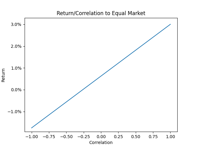
On the rightmost point of this line, we see that if an asset is perfectly correlated to global equities, then we require it to have the same return. (In effect, this point represents the equity market itself.) At the other extreme, if an asset is perfectly anti-correlated with equities, it can have a return as low as –1.75% and still be worth investing in. In the middle, an asset with zero correlation must earn an expected return of 0.62%.

This line¹⁷ has a slope of 2.38. That means if we can increase return by (say) 0.238% while increasing correlation by less than 0.1, then we should do it, and vice versa.

As another example, suppose we can invest in leveraged VMOT¹⁸, which has the same volatility as global equities, an expected return of 7%, and a correlation of 0.5. Holding volatility fixed, what return/correlation would another asset need to have to match the expected value of VMOT?

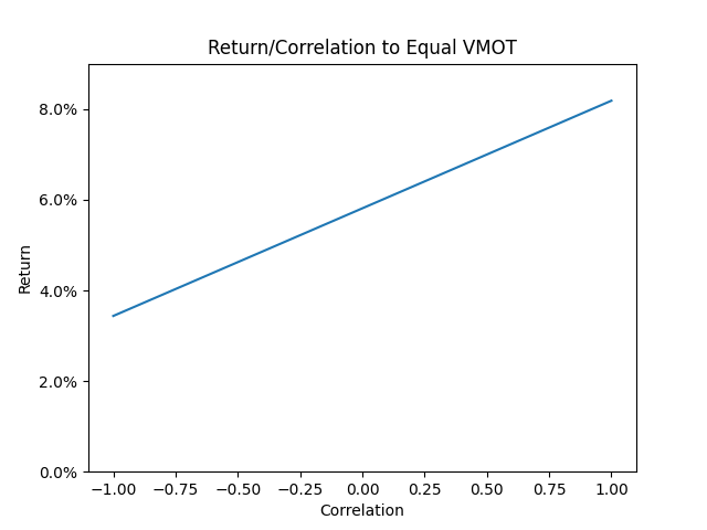
For an asset with perfect correlation to global equities, we would demand a return of 8.19%. For an uncorrelated asset, we would accept a return of 5.81%. And for an asset with a perfect negative correlation, the expected return can go as low as 3.44%.

Impact of assumptions

The analysis in this essay made a number of assumptions. How realistic are they? If we change them, how might the results change?

Leverage and shorts are free

So far, we have assumed that we can get leverage at the risk-free rate and shorts for free. But this is usually not true in practice. Let’s take the more realistic assumptions that leverage costs 1% on top of the risk-free rate, and short positions cost 0.25%.¹⁹

This gives the following asset allocation:

Allocation
Market	–38%
Val/Mom	39%
VMOT	115%
ManFut	50%

Summary Statistics
Total Altruistic Return	3.08%
Personal Return	7.92%
Personal Standard Deviation	20%
Personal Correlation to Market	0.32

Notice that the short market position is smaller than before: –38% instead of –76%. This portfolio also has a smaller long position (204% instead of 226%). Interestingly, it actually increases the allocation to VMOT. This happens because Market has a stronger correlation to Val/Mom than to VMOT, so when the optimizer reduces the size of the short position, it no longer cancels out the high correlation of Val/Mom, so it prefers to shift some money to an asset with lower correlation.

For comparison, the optimal self-interested asset allocation looks like this:

Allocation
Market	0%
Val/Mom	42%
VMOT	95%
ManFut	42%

Summary Statistics
Total Altruistic Return	N/A
Personal Return	8.33%
Personal Standard Deviation	20%
Personal Correlation to Market	0.58

This allocation eschews short positions entirely.

We control only a small portion of the total altruistic portfolio

So far we have assumed that, in total, other value-aligned altruists donate much more money than we do. (Specifically, my calculations assumed we control 1% of the overall portfolio, although the exact number doesn’t matter much.)

If we control a large fraction of the altruistic portfolio—e.g., if we manage a large foundation, or if we donate to a cause that receives almost no attention—then our portion of the altruistic portfolio should look much more similar to the optimal overall altruistic portfolio. Specifically, that means:

1. We should care less about reducing correlation to other altruistic investors.
2. We might not want to get as much leverage as possible, instead getting an amount that’s closer to the overall optimum level.

Assets follow log-normal distributions

I’m using standard deviation as the measure of risk. That only works if asset prices follow log-normal distributions. In practice, most assets have a left-skewed distribution, meaning they see very bad performance more often than a log-normal distribution would predict.

Therefore, standard deviation does not properly capture the risk of most assets. You should usually use less leverage than you’d think just from looking at the standard deviation. (In a previous essay, I compared theoretically optimal leverage (over log-normally distributed assets) to the (simulated) historical performance of leveraged portfolios. Over the asset classes I examined, theoretically optimal leverage somewhat overestimated truly optimal leverage, but not by a huge margin.)

Usually, people don’t actually care about the standard deviation of a portfolio: they care about drawdowns. I like the ulcer index as a way to measure the tendency of a portfolio to experience drawdowns. Unfortunately, we can’t easily run an ulcer index minimization algorithm, because that would require having full price data of each asset, not just the return/volatility/correlations. Even if we do have full price data, the results would be highly sensitive to which particular drawdowns occurred during the sample period.

We discussed optimal portfolios under leverage constraints and risk (i.e., standard deviation) constraints. But perhaps a more better approach is to use a drawdown constraint. Assume I can only accept, say, a 90% drawdown on my altruistic investments. What maximum drawdowns do I expect from each asset, and how likely are the different assets to experience big drawdowns at the same time? Then I can use this to derive an optimal portfolio. This is approximately how I decide on an asset allocation in my personal account (although I certainly have a much lower drawdown tolerance than 90% on my personal funds!). I’m not sure how to formalize this, so I just make ad-hoc estimations.

It should be noted that some assets do not skew left. Importantly, managed futures have historically been right-skewed. For example, Chesapeake Capital’s managed futures fund⁶ experienced a standard deviation of 19% from 1988–2019, as compared to the US stock market’s 14%. But the Chesapeake fund performed substantially better on other measures of risk:

	Chesapeake	US Equities
Skewness	0.86	–0.67
Max Drawdown	32%	50%
Ulcer Index	10.5	14.2

(Notably, Chesapeake experienced its maximum drawdown not in 2007–2009 like US equities, but in 2010–2013, while the market was going up.)

If we expect this to continue in the future, then standard deviation is actually too conservative a measure of risk for assets like this one.

Asset correlations are stable over time

In ordinary times, stocks, commodities, and real estate have fairly low correlations to each other. But in bad times, correlations tend to go to 1. During the recession of 2008, all three asset classes experienced large drawdowns at the same time. So even if we build a diversified portfolio, that diversification might fail us at exactly the wrong time.

Some assets and strategies, most notably trendfollowing (including managed futures), have actually shown positive return during equity drawdowns.²⁰ Including such strategies can help alleviate concerns about correlations increasing during market downturns.

Optimization techniques can predict optimal future asset allocations

This essay implicitly assumed that we can use techniques such as geometric mean maximization to derive optimal asset allocations. But substantial literature has shown that the related technique of mean-variance optimization (MVO) tends to over-fit to past results and does a bad job of estimating forward-looking optimal portfolios—in fact, it maximizes estimation error (Michaud, 1989²¹). Geometric mean maximization does a better job than MVO of predicting out-of-sample performance (Estrada, 2010³), but still isn’t entirely reliable.

In my analysis, I used future return projections rather than naively taking historical returns, which should fix the problem of over-fitting to historical performance. But this still requires my estimates to be (reasonably) accurate, which they might not be.

Some more complex methods, such as Bayesian methods and portfolio resampling, can incorporate uncertainty into the portfolio optimization process (Fuhrer and Hock, 2019²²). These methods generally favor more diversified portfolios: if you don’t know which assets will perform best in the future, it makes sense to hedge your bets.²³

Ultimately, the takeaway from this essay should not be that a particular allocation shown is close to optimal. We should focus on the general principles rather than specific numbers—for example, the principle that altruistic investors should probably short the market, but their short position should be smaller than their long positions.

Altruists have logarithmic utility

Investors with logarithmic utility functions want to maximize geometric mean. So by focusing on the geometric mean, I have implicitly assumed that altruists have logarithmic utility. This seems at least approximately true, but it might not be true exactly. If altruists experience more rapidly diminishing marginal utility, then they want to diversify more than this essay suggests, and vice versa.

(Note that self-interested individuals are probably more risk averse than logarithmic utility would suggest. It seems plausible that altruistic endeavors on the whole are less risk-averse than individuals.)

Conclusions

In brief:

• If most altruists don’t use enough leverage, or under-allocate to the assets with highest expected return, then the top priority is to get a (leveraged) allocation to the high-return assets.
• The optimal allocation probably includes a modest short position to reduce correlation to the typical altruistic portfolio.
• If altruists do use enough leverage but don’t fully diversify, then altruists on the margin should invest in diversifying assets, perhaps exclusively.

In practice, it seems most likely that altruists do under-allocate to the value, momentum, and trend factors, as well as some high expected return markets like emerging-country equities. This suggests that, on the margin, altruists should hold whichever investments they believe have the highest expected return, while shorting over-subscribed markets such as US equities.

How has writing this essay changed my mind?

Previously, I was moderately convinced by the theoretical argument (given here) that altruistic investors should exclusively hold uncorrelated investments. I wasn’t sure this was true in practice, because I suspected that the overhead costs of maintaining market-neutral long/short positions would exceed the benefits.

The analysis in this essay somewhat justifies my practical concerns, although I was right for the wrong reason. Yes, the costs of leveraged and short positions do make such positions somewhat less appealing, but not much. More importantly, if you believe that most altruistic investors use insufficient leverage or under-weight the highest-return assets, then—at least according to the analysis in this essay—you should primarily invest in the assets with highest expected (geometric) return, even if they’re not uncorrelated with typical investments. In particular, investors who can’t use leverage may simply want to invest in whichever asset has the highest expected return, without regard to its volatility or correlation.

Calculations for this essay were done using mvo.py.

Appendix

Appendix A: Derivation of mean/standard deviation/correlation estimates

Mean, standard deviation, and correlation for global equities, US equities, international equities, commodities, and bonds are based on forward projections from Research Affiliates’ Asset Allocation Interactive. Accessed 2020-11-27.

Means for Val/Mom, VMOT, and ManFut were derived by taking historical return in excess of the market, adding expected market return, subtracting projected costs, and dividing the premium in half based on the assumption that value, momentum, and trendfollowing will work less well in the future than they have in the past.

Baseline historical returns for Val/Mom and VMOT are taken from a 20-year backtest by Alpha Architect and my own 90-year backtest using the Ken French Data Library. Baseline historical returns for ManFut are taken from Moskowitz et al. (2012)⁸ and Hurst et al. (2014)¹².

Standard deviations for Val/Mom and VMOT are taken from the same backtests with no adjustments, on the basis that we have no reason to expect future volatility to be higher or lower than it was in the past.

Standard deviation for ManFut comes from the fact that high-volatility managed futures mutual funds generally target about a 15% standard deviation.

Correlation matrix was calculated with a backtest using the Ken French Data Library and AQR’s Time Series Momentum: Factors, Monthly data set, on the assumption that future correlations will resemble historical correlations. I revised some of the correlations slightly downward because my backtest only included US stocks, but an actual portfolio would include globally diversified stocks. Managed futures correlations were validated using the actual historical performance of the Chesapeake Capital managed futures fund, 1988–2019.

Appendix B: Sensitivity analysis of risk-constrained allocation

Variations on Market + Val/Mom + VMOT + ManFut

Asset allocation with maximum 40% standard deviation, but return expectations unchanged

Allocation
Market	–145%
Val/Mom	171%
VMOT	164%
ManFut	114%

Summary Statistics
Total Altruistic Return	3.20%
Personal Return	14.65%
Personal Correlation to Market	0.23

Asset allocation with 1% excess return for each factor (Val/Mom return = 4%, VMOT return = 3%, ManFut return = 1%)

Allocation
Market	–62%
Val/Mom	141%
VMOT	11%
ManFut	68%

Summary Statistics
Total Altruistic Return	3.05%
Personal Return	4.70%
Personal Correlation to Market	0.44

Asset allocation with 0% excess return for each factor (Val/Mom return = 3%, VMOT return = 2%, ManFut return = 0%)

Allocation
Market	20%
Val/Mom	62%
VMOT	50%
ManFut	50%

Summary Statistics
Total Altruistic Return	3.03%
Personal Return	3.54%
Personal Correlation to Market	0.72

Asset allocation when other altruists invest 100% of their money into VMOT

Allocation
Market	–45%
Val/Mom	102%
VMOT	47%
ManFut	64%

Summary Statistics
Total Altruistic Return	5.92%
Personal Return	9.16%
Personal Correlation to VMOT	0.45

Asset allocation when other altruists invest all their money into VMOT, with optimal leverage (405%), and allowing us to use up to 52% standard deviation (so that we can match 405% leverage)

Allocation
Market	–189%
Val/Mom	430%
VMOT	–121%
ManFut	270%

Summary Statistics
Total Altruistic Return	16.02%
Personal Return	14.70%
Personal Standard Deviation	52%
Personal Correlation to VMOT	0.62

Same, but only allowing us a 20% standard deviation

Allocation
Market	–73%
Val/Mom	166%
VMOT	–47%
ManFut	104%

Summary Statistics
Total Altruistic Return	15.94%
Personal Return	7.91%
Personal Standard Deviation	20.00%
Personal Correlation to VMOT	0.62

Asset allocation with more optimistic expectations for managed futures (ManFut return = 5%)

Allocation
Market	–75%
Val/Mom	104%
VMOT	41%
ManFut	85%

Summary Statistics
Total Altruistic Return	3.11%
Personal Return	10.12%
Personal Correlation to Market	0.20

Asset allocation with highly optimistic expectations for managed futures (ManFut return = 10%)

Allocation
Market	–66%
Val/Mom	112%
VMOT	–16%
ManFut	119%

Summary Statistics
Total Altruistic Return	3.16%
Personal Return	14.65%
Personal Correlation to Market	0.14

Asset allocation using historical performance, net of estimated costs (market return = 5%, Val/Mom return = 12%, VMOT return = 12%, ManFut return = 9%, ManFut standard deviation = 10%)

Allocation
Market	–82%
Val/Mom	125%
VMOT	13%
ManFut	142%

Summary Statistics
Total Altruistic Return	5.17%
Personal Return	22.40%
Personal Correlation to Market	0.19

Variations on US + International + Commodities + Bonds

Asset allocation when US equities return 5%

Allocation
US Market	82%
International	37%
Commodities	11%
Bonds	–30%

Summary Statistics
Total Altruistic Return	4.07%
Personal Return	6.02%
Personal Correlation to Altruistic Portfolio	0.99

Asset allocation when bonds return –3%

Allocation
US Market	–225%
International	263%
Commodities	5%
Bonds	58%

Summary Statistics
Total Altruistic Return	0.82%
Personal Return	10.16%
Personal Correlation to Altruistic Portfolio	0.30

Asset allocation when bonds have 0.0 correlation to each other asset

Allocation
US Market	–247%
Global ex-US	269%
Commodities	–7%
Bonds	84%

Summary Statistics
Total Altruistic Return	1.19%
Personal Return	10.90%
Personal Correlation to Altruistic Portfolio	0.19

Notes

1. The effective altruism movement, and charity in general, are over-represented in the United States.
2. Most investors over-weight investments within their own country.
3. Some altruistic investors probably hold something like a “standard” 60/40 stocks/bonds portfolio, and others probably hold stocks only. So maybe it averages out to around 80/20.