Summary

Last updated 2022-04-15; see Errata.

Confidence: Highly likely.

Some altruists are much less risk-averse than ordinary investors, and may want to use leverage. But foundations and donor-advised funds legally cannot access most forms of leverage. As an alternative approach, leverage-constrained investors could buy concentrated positions in small-cap value and momentum stocks. For example, instead of buying an ETF that holds the best half of the market as ranked by value or momentum, they could buy the top 10%.

According to backtests, when portfolio concentration increases, both return and risk increase, and return increases more than risk (so that concentrated portfolios have higher risk-adjusted returns).

Large investors cannot hold concentrated portfolios without moving the market, so they probably prefer to use leverage if they can. Small investors probably prefer to buy concentrated investments because they offer higher risk-adjusted returns than leveraged broad portfolios.

Disclaimer: This should not be taken as investment advice. Any given portfolio results are hypothetical and do not represent returns achieved by an actual investor.

Contents

• Summary
• Contents
• Motivation
• Known approaches
• Increasing expected return via concentration
• Fees, transaction costs, and taxes
• How does concentrated investing compare to using leverage?
• On future expectations
• Finding concentrated ETFs
• Errata
• Appendix A: Significance tests
• Appendix B: Replication on international equities
• Appendix C: Factor regression on selected portfolios
• Notes

Motivation

Some investors cannot use leverage. For example, foundations, donor-advised funds, and IRAs are prohibited from using certain types of investments, including margin loans. Other investors have access to leverage, but have to pay high fees to get it. But sometimes, investors want to increase their return and risk. Can we do that without explicitly using leverage?

Known approaches

Some stocks are more volatile than others. One way to simulate leverage might be to buy stocks with high volatility. Unfortunately, this doesn’t work: high-vol stocks do not provide enough return to justify the higher risk.¹² This may happen because leverage-constrained investors already overpay for stocks with high volatility.

As a different approach, we could tilt toward small-cap, value, and momentum stocks. These tilts all tend to increase both risk and return.³⁴⁵⁶ (Gordon Irlam has proposed that altruists use small-cap value rather than leverage as a (sometimes) better method of increasing return.) Most funds that implement these tilts hold around half to a third of the total market, and end up with a little bit higher volatility and expected return than the market, but not much higher.

Increasing expected return via concentration

Small-cap stocks, value stocks, and especially small-cap value stocks tend to earn higher return (and higher risk) than the broad market. Small-cap and value index funds typically hold about half the market. Can we enhance our return⁷ by concentrating in a narrower corner of the market, such as 10% instead of 50%?

Let’s use the Ken French Data Library to look at portfolios formed on size, value, and momentum at various levels of concentration.

Ignoring size for now, did more concentrated value and momentum portfolios historically perform better?

The chart below shows historical returns for US stocks using three valuation metrics and one momentum metric:

• value: book to market (B/M)
• value: earnings to price (E/P)
• value: cash flow to price (CF/P)
• momentum: 12-month return, excluding the most recent month (Mom)

It includes both equal-weighted (EW) returns (where each stock receives the same weight) and value-weighted (VW) returns (where stocks are weighted in proportion to market cap).⁸

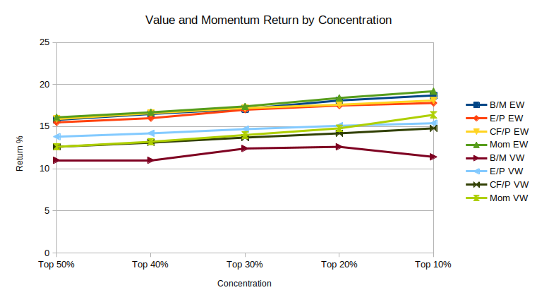
For each of the four metrics, return monotonically increased with concentration (with the sole exception of B/M value-weighted moving from top 20% to top 10%).

Let’s narrow in on value stocks as measured by B/M. The next chart shows B/M returns over the total market as well as over small caps (defined as the 10% smallest stocks):⁹

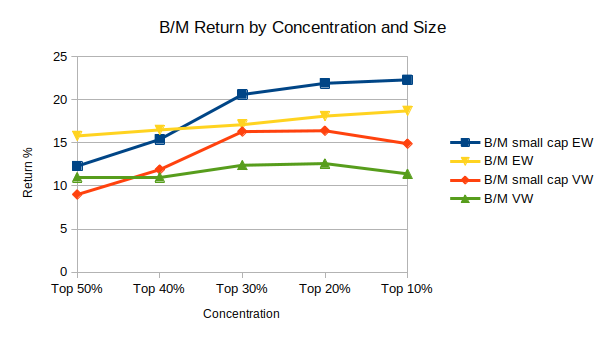
We see a similar pattern, where more concentration means higher return. Within small caps, this pattern has a steeper slope, and small-cap value stocks consistently outperformed all-cap value stocks except at the weakest level of concentration. Relatedly, equal-weighting outperformed value-weighting—equal-weighting gives relatively more weight to small caps, so this is a different form of small cap tilt.

Most off-the-shelf value and momentum funds hold about half the market, value-weighted. If instead of buying one of those funds, we held only the top 10% and used equal weighting, historically we could have increased returns by a lot:

	50% VW	10% EW	Improvement
B/M	11.0%	18.7%	7.7%
E/P	13.8%	17.8%	4.0%
CF/P	12.6%	18.1%	5.5%
Mom	12.6%	19.2%	6.6%

As return increased with concentration, volatility increased at a similar pace. Equal-weighted portfolios had higher risk-adjusted returns across the board than their value-weighted counterparts; but equal-weighted portfolios had similar risk-adjusted returns at all levels of concentration (including 50%, 40%, 30%, 20%, and 10%).

These differences in returns across concentration, market cap, and weighting are highly statistically significant, as are the differences in volatility (see Appendix A).

The following table shows the risk-adjusted returns (Sharpe ratios) for value and momentum portfolios:

	50% VW	10% EW	Improvement
B/M	0.45	0.57	0.12
E/P	0.71	0.74	0.03
CF/P	0.63	0.71	0.08
Mom	0.57	0.73	0.16

We can get higher returns (accompanied by higher risk) by going even deeper into small-cap value and momentum. According to some backtests I ran on a different (non-public) data set, a portfolio of the top 30 value stocks (equal-weighted) would have historically returned about 30% per year gross of costs, with a standard deviation of about 45%. This is similar to the historical performance of a US total market index with 3:1 leverage. However, this portfolio would mainly have consisted of very small stocks (market cap $200 million or less), so trading costs could destroy a lot of the value of this strategy in practice.¹⁰

Fees, transaction costs, and taxes

So far, I have focused on gross returns. But real-world strategies have to pay various costs, including management fees, trading costs, and taxes. How much do these matter?

I did not find much published research on real-world transaction costs and I only have limited personal experience trading individual stocks, so take the following with a grain of salt.

Investors with less than $1 million probably shouldn’t worry about transaction costs. Even micro-cap stocks (with market caps between $50 million and $200 million) are liquid enough that small investors will probably end up paying 0.25% or less per trade. If you buy value stocks and rebalance once a year, transaction costs will probably be low enough not to matter. Momentum requires more frequent rebalancing, so even small investors might prefer to restrict themselves to some minimum market cap threshold (somewhere in the $200 to $500 million range) or take other measures to reduce costs.

Larger investors must take care not to move the market when they buy and sell stocks. Investors with substantially more than $1 million might prefer not to trade micro-cap stocks. Investors with much more money (perhaps around $100 million) can’t use equal weighting because they will move the market too much if they try to put substantial positions into small-caps.¹¹

If you hire an investment manager to run a strategy like this, they will charge a fee—probably around 1% per year. This dampens the value of investing in a concentrated portfolio rather than simply buying an off-the-shelf mutual fund or ETF. Or you could manage your own portfolio, avoiding the fee but giving yourself more work to do. I used to manage my own concentrated portfolio of value stocks, and it took me two hours of work per year. A momentum strategy would probably require somewhere around 10–20 hours per year. But if you manage the portfolio yourself, you need to be confident that you won’t make trading mistakes.

Value and momentum portfolios both have some turnover, and turnover means you pay taxes on gains. The more concentrated a strategy, the more turnover it has. This may be prohibitive for taxable investors, who will pay substantial taxes if they have to sell positions regularly.¹² Taxable investors could avoid turnover by buying an ETF that uses an appropriately concentrated strategy. ETFs charge fees, and concentrated funds tend to have substantially higher fees than broad ETFs. But these fees are probably still lower than the cost of hiring an investment manager, and lower than the tax drag from trading individual stocks.

How does concentrated investing compare to using leverage?

Adding leverage to a portfolio increases both return and volatility while keeping risk-adjusted return the same (before costs). In the backtests we looked at, more concentrated portfolios had both higher returns and higher risk-adjusted returns.

Two other important considerations:

1. Small investors have no difficulty buying an equal-weighted portfolio of small-cap stocks. Large investors cannot buy small-caps without moving the market.
2. Small investors face relatively high costs of leverage. Large investors can take advantage of their size to get leverage more cheaply.

These considerations suggest that small investors should invest in concentrated portfolios while large investors should use leverage.

Under some conditions, small investors may still prefer to hold leveraged broad portfolios if they can, mainly for two reasons:

1. Manually managing a basket of stocks is both less tax-efficient and more time-consuming than buying and holding an ETF (or group of ETFs) and applying leverage.
2. The analysis in this essay only considered stock portfolios. Adding bonds, real assets, or other factors might improve an investor’s overall risk-adjusted return.

On future expectations

So far, we have looked at simulated historical performance of different strategies. That doesn’t tell us how these strategies will perform in the future.

We care about two questions:

1. Will value/momentum investing continue to outperform the market?
2. Will concentrated value/momentum investing continue to beat the market, and continue to beat diversified value/momentum investing?

The first question has been addressed elsewhere in detail. For a deep dive into arguments on why value investing might not work anymore and why they’re probably wrong, see Israel, Laursen & Richardson (2020), Is (Systematic) Value Investing Dead? and Cliff Asness’ (less rigorous, easier to read) article of the same name. The future of momentum investing is much less clear. Israel & Moskowitz (2013)’s The Role of Shorting, Firm Size, and Time on Market Anomalies provides at least some reason to expect momentum’s outperformance to persist, but no strong evidence.¹³

For the second question, if we expect value and maybe momentum to persist, then we should probably expect concentrated portfolios’ even better performance to persist for the same reasons. In fact, the argument that concentrated value/momentum will persist appears even stronger. If strategies like value and momentum become more popular among large sophisticated investors, then they will tend to perform worse. But large investors cannot buy equal-weighted small cap portfolios. And small investors who do use value/momentum typically invest via broad mutual funds or ETFs, not concentrated baskets of stocks.

As a counterpoint, just because a strategy has higher risk doesn’t mean you’re compensated for that risk. For example, a basket of 30 randomly-chosen stocks is riskier than an index fund, but doesn’t have higher expected return.¹⁴ Investing in concentrated value/momentum portfolios only makes sense if they’re able to outperform randomly-chosen concentrated portfolios.

Finding concentrated ETFs

The etf.com screener can be used to identify concentrated ETFs. For example, the following table lists every ETF filtered by “Strategy: Value” and “Weighting Scheme: Equal”. This list does not include every concentrated value ETF because (a) some funds are concentrated but not equal-weighted, and (b) some funds don’t have sufficiently detailed metadata on etf.com to show up in these screens. I attempted to estimate concentration by comparing the number of stocks in each fund to the underlying index, but the numbers might not be fully accurate.

ETF	Region	Market Cap	Concentration
EEMD	emerging markets	mid+large	10%
IVAL	developed ex-US	mid+large	5%
QVAL	US	mid+large	5%
SPDV	US	mid+large	10%
SVAL	US	small	12.5%

Disclosure: I invest in QVAL and IVAL.

Errata

2022-04-15:

The original version of this post claimed that concentrated and broad factor portfolios have similar risk-adjusted returns. That is incorrect: equal-weighted concentrated portfolios have higher risk-adjusted returns than value-weighted broad portfolios.

Originally, I calculated the Sharpe ratio using the geometric mean, that is, (geometric mean - risk-free rate) / standard deviation. I should have calculated it using the arithmetic mean: (arithmetic mean - risk-ree rate) / standard deviation. The geometric Sharpe ratio understates the difference in risk-adjusted return between (relatively) low-volatility and high-volatility portfolios.

This change suggests that small investors should favor concentrated portfolios over leveraged broad portfolios even if they have access to cheap leverage.

I added a new table to report Sharpe ratios for various portfolios. I also corrected the table in Appendix B and updated it to include historical data through 2022-02.

Appendix A: Significance tests

This table shows p-values for the excess return of top 10% equal-weighted over top 50% value-weighted for various metrics.¹⁵¹⁶

• Tested using monthly data.
• Calculated over log returns on the assumption that log returns follow a normal distribution.
• Using a two-sided T-test on the null hypothesis that the excess return of the concentrated portfolio is zero.

metric	mean	stdev	n	p-val
B/M	0.66	5.401	1132	3.2e-5
E/P	0.32	3.294	832	6.8e-3
CF/P	0.43	3.536	832	6.4e-4
Mom	0.53	3.615	1119	9.6e-7

Interestingly, among the two null hypotheses

1. a concentrated factor portfolio has the same return as a broad factor portfolio, and
2. a concentrated factor portfolio has the same return as the broad market,

the first hypothesis is rejected much more strongly. This happens because the two factor portfolios are highly correlated, so their difference has a relatively low standard deviation.

The excess returns of (a) top 10% VW over top 50% VW, (b) top 10% EW over top 50% EW, (c) top 50% EW over top 50% VW, and (d) top 10% EW over top 10% VW were generally statistically significant, but to a lesser degree. The next table gives p-values for these four portfolio differences using each of the four factors:

		B/M	E/P	CF/P	Mom
10% VW	50% VW	0.28	0.08	0.03	2e-4
10% EW	50% EW	2e-3	2e-3	3e-3	2e-4
50% EW	50% VW	2e-5	0.06	3e-3	1e-4
10% EW	10% VW	2e-5	0.11	0.03	0.03

(9 out of 16 are significant at p=0.01, and 5 are significant at p=0.001.)

This suggests that both methods of increasing concentration (moving from 50% to 10%, and from value-weight to equal-weight) by themselves increased return.

The next table shows p-values from significance tests for standard deviation over B/M (equal-weighted). Differences in standard deviations between portfolios were highly significant.

• Tested using monthly data, n=1132.
• Differences in standard deviations were tested using a two-sided F-test.

		p-val
50% BM	10% BM, small 10%	1e-22
50% BM	10% BM	1e-11
30% BM	10% BM	1e-6
10% BM	10% BM, small 10%	1e-8
30% BM	30% BM, small 10%	1e-10

Caveat #1: These t-tests assume that stock returns follow a normal distribution. Although this is a common assumption, it’s not quite accurate, as stocks tend to experience tail events more frequently than a normal distribution would predict. That means the “true” p-values are higher than what’s reported above, and the lower the reported p-value, the more wrong it is. For example, at one point the concentrated B/M portfolio experienced an excess drawdown of 43% over a 10-month period, which “should” only happen once every 21,000 years.¹⁷ (Similarly, US equities “should” experience an 80% drawdown only once every 70,000 years, and yet it happened during the Great Depression.)

Caveat #2: I am not particularly well-versed in significance testing, so I could have made mistakes in these calculations.

Appendix B: Replication on international equities

The Ken French Data Library only includes international equity returns back to 1990 (instead of 1926), and only reports value/size quintiles rather than deciles. So this international replication is more limited, but it illustrates the same patterns.

This table gives summary statistics for a variety of equal-weighted and value-weighted portfolios on B/M and size at various levels of concentration. As with US equities, geometric return increased with higher concentration, smaller size, and equal weighting. These three relationships were all statistically significant at p<0.001, even when excluding the first portfolio in the table (which had a much higher return than the others).¹⁸¹⁹

	Sharpe ratio	Return	Standard Deviation
20% BM, small 20% EW	0.97	18.1%	16.3%
20% BM EW	0.50	10.2%	17.5%
40% BM, small 40% EW	0.62	11.6%	16.3%
40% BM EW	0.47	9.2%	17.0%
20% BM, small 20% VW	0.63	11.4%	15.4%
20% BM VW	0.40	8.1%	16.9%
40% BM, small 40% VW	0.48	9.0%	15.5%
40% BM VW	0.39	7.7%	16.3%

Appendix C: Factor regression on selected portfolios

This table provides a monthly time series factor regression on several portfolios, using factors as defined in the Ken French data library.

• Beta: market beta factor.
• SMB: size factor.
• HML: value factor.
• Alpha: excess return not explained by these three factors.
• P-values are reported for the null hypothesis that alpha = 0.
• I use 30% as the diversified portfolio rather than 50% because I cannot fully accurately construct a 50% value-weighted portfolio using the Ken French data. For the data on historical returns, I wasn’t concerned about this because it doesn’t make much difference; but for a factor regression, I want to be as accurate as possible.

	Beta	SMB	HML	Alpha	p-val
30% BM VW	1.07	0.22	0.79	-0.05	0.07
10% BM VW	1.18	0.55	1.08	-0.23	0.002
10% BM, small 10% VW	0.97	1.57	1.14	0.05	0.74
30% BM EW	1.01	1.06	0.85	0.24	2e-5
10% BM EW	1.03	1.33	1.11	0.31	0.004
10% BM, small 10% EW	0.97	1.71	1.21	0.59	0.0008

Based on this limited sample, it appears that more concentrated portfolios do not have higher market beta, but do tend to have greater exposure to the size and value factors, as well as higher alpha. Most notably, the equal-weighted portfolios have more alpha than the value-weighted ones.

If we add leverage to the 30% VW portfolio in an attempt to replicate a more concentrated portfolio like 10% EW, the former will have less alpha and more market beta. This may be undesirable in the context of a broader portfolio that includes other allocations to equities.

I found this result surprising. I would have predicted that concentrated portfolios’ higher return would primarily come from higher factor exposure, especially exposure to the value factor (HML). While my prediction is at least partially true, even the most concentrated portfolio only had 1.21x loading on HML, and a significant portion of the outperformance could not be explained by any factor.

Conventionally, HML is defined as the return of the top 30% of value stocks minus the bottom 30%, value-weighted. If we redefine HML as the top 30% minus the bottom 30% equal-weighted (keeping the other factor definitions the same), we get an interesting result:

	Beta	SMB	HML EW	Alpha	p-val
30% BM VW	1.13	0.03	0.53	-0.21	8e-5
10% BM VW	1.26	0.27	0.78	-0.47	9e-8
10% BM, small 10% VW	1.03	1.15	1.08	-0.37	0.004
30% BM EW	1.06	0.79	0.72	-0.02	0.7
10% BM EW	1.09	0.96	0.99	-0.06	0.6
10% BM, small 10% EW	1.02	1.24	1.23	0.09	0.6

We can see that higher factor loadings on SMB and HML EW fully explain the return of the more concentrated portfolios. Meanwhile, the value-weighted portfolios have statistically significant negative alpha.

One possible explanation is that switching from value-weighting to equal-weighting “unlocks” more of the value premium by allowing investors to assign relatively higher weight to the most undervalued stocks, and this component of the value premium is invisible to HML VW.

The other value metrics, E/P and CF/P, exhibit a similar effect: when we regress on a value-weighted HML factor using E/P or CF/P (instead of B/M), the equal-weighted portfolios have statistically significant alpha at p<0.001, with 10% EW having more alpha than 30% EW. On an equal-weighted HML factor, value-weighted portfolios have negative alphas, but none are statistically significant at p<0.001 (or even p<0.01).

The following table gives factor regressions for selected momentum portfolios. “Mom” is the momentum factor.

	Beta	SMB	Mom	Alpha	p-val
30% Mom VW	1.07	0.08	0.37	0.03	0.35
20% Mom, small 20% VW	1.09	1.32	0.23	0.44	1e-4
30% Mom EW	1.03	0.74	0.27	0.31	1e-11
10% Mom EW	1.11	0.94	0.45	0.28	1e-5
20% Mom, small 20% EW	1.05	1.38	0.17	0.65	1e-6

Here we see qualitatively similar results to the first table, where more concentrated portfolios tend to have stronger exposure to the size and momentum factors, as well as significantly positive alpha.

When we use an equal-weighted momentum factor instead of value-weighted, concentrated portfolios still have statistically significant alpha. However, when we replace the momentum factor with an equal-weighted long-only factor (that is, 30% Mom EW minus the risk-free rate), none of the momentum portfolios have alpha (either positive or negative).²⁰ Relatedly, while equal-weighted momentum portfolios did earn higher risk-adjusted returns than comparable value-weighted strategies, the difference was not as large as for B/M. These two observations suggest that switching from value-weighting to equal-weighting does not matter as much for momentum as it does for value. This makes intuitive sense: equal-weighting implicitly tilts toward small-cap value, so it unlocks more of the value premium, but there’s no reason to expect it to do the same for momentum.

Notes